CMU 15719/18709 Advanced Cloud Computing S25 学习笔记

L00 Cloud Computing

(& P01.1 - The NIST Definition of Cloud Computing & P01.2 - A View of Cloud Computing)

Cloud Computing - Essential Characteristics:
1. On-demand self-service
2. Broad network access
3. Resource pooling: resources are pooled, dynamically assigned and reassigned, the customer has no knowledge over the exact location of the provided resources (but can specify location at a higher level of abstraction, e.g., country, state, or datacenter)
4. Rapid elasticity
5. Measured service
Cloud Computing - Service models:
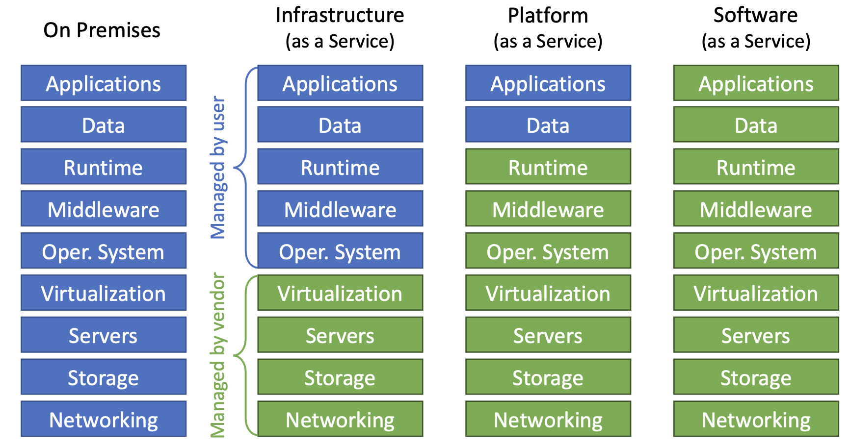
1. Software as a Service SaaS
2. Platform as a Service PaaS (e.g. Google AppEngine): The capability provided to the consumer is to deploy onto the cloud infrastructure consumer-created or acquired applications created using programming languages, libraries, services, and tools supported by the provider. The consumer does not manage or control the underlying cloud infrastructure including network, servers, operating systems, or storage, but has control over the deployed applications and possibly configuration settings for the application-hosting environment.
3. Infrastructure as a Service IaaS (e.g. AWS EC2): Basic hardware model with all (virtual) resources exposed
Cloud Computing - Deployment models:
1. Private cloud
2. Community cloud: providers and consumers are different organizations with strong shared concerns (federations, such as “U.S. hospitals”)
3. Public cloud
4. Hybrid cloud
Cloud Computing - benefits:
1. The appearance of infinite computing resources available on demand, quickly enough to follow load surges, therby eliminating the need to plan far ahead for provisioning
2. The elimination of an up-front commitment by cloud users, thereby allowing start small
3. The ability to pay for use of computing resources on a short-term basis as needed, thereby rewarding conservation
Cloud Computing Services - tradeoff:
1. Lower Level Abstraction: e.g. Hardware virtual machines like EC2
  - enable more specialization to app-specific goals
  - semantics and management issues are application-dependent => difficult to offer automatic scalability and failover
2. Higher Level Abstraction: e.g. Application frameworks (Application domain-specific platforms) like Google AppEngine
  - simplify matching user tasks and free users from details of provisioning, configuration, fault tolerance, etc.
  - clean separation of computation, storage, and communication => impressive autoscaling and high-availability mechanisms
Cloud Computing - Obstacles:
1. Privacy & security
2. Utility issues (service availability, provider trust, etc.)
3. High cost of networking (data transfer) combined with always remote
4. Performance unpredictability
5. in situ development/debugging: Bugs often appear only at scale, in the situation of use (in situ)
6. Consumer reputation shared with other consumers - need trusted auditor
7. Software licensing - $/yr/CPU is not elastic and pay as you go

L01 - Elasticity

(& P01.3 Dynamically Scaling Applications in the Cloud)

1. Load Balancer: partitions requests among server machines

Load balancing approaches
- DNS load balancing
  - PRO: out of band of actual TCP/HTTP requests
    - can distribute arbitrary bandwidth (not limited by bandwidth of a router)
    - scales better, cheaper, easier to implement
  - PRO: lower latency because there is no extra component (the load balancer) doing some processing on communication between clients and servers
  - CON: takes a long time to change
    - Tells client a binding of a name to an IP (list), which makes dynamic changing of the binding hard, or at least up to the client (specifically, clients could continue using an outdated IP address until the cache expires)
    - Also, network middleboxes may cache answer for many clients
- Having “Router” distribute TCP connection open packets
  - have one IP address for entire web service, which goes to a “load balancing” router, and have that router spread SYN packets sent to web server among different server machine
  - PRO: router doesn’t have to think or remember too much
  - CON: all client<->server network traffic must go through the router
  - CON: decision is for entire connection lifetime which could be too long to do good balancing
- Having “Router” distribute individual requests embedded in connections
  - Have router be endpoint for TCP connection and interpret the bytes, Router opens connections to all internal servers, to forward reqs and receive replies
  - PRO: most dynamic approach
  - CON: requires the most processing and state in the router
Load balancer - Liu & Wee’s “Rule of Thumb”:
- CPU-intensive applications: Use a LB to distribute computation across instances.
- Network-intensive applications: Prefer a powerful standalone instance over multiple VMs (no LB)
- Highly network-intensive applications: Use DNS-based load balancing to avoid single-instance bandwidth limits.

2. Elasticity

Scale Out (Horizontal scaling) vs. Scale Up (Vertical scaling)
Server Scalability: How is elasticity provided to web servers?
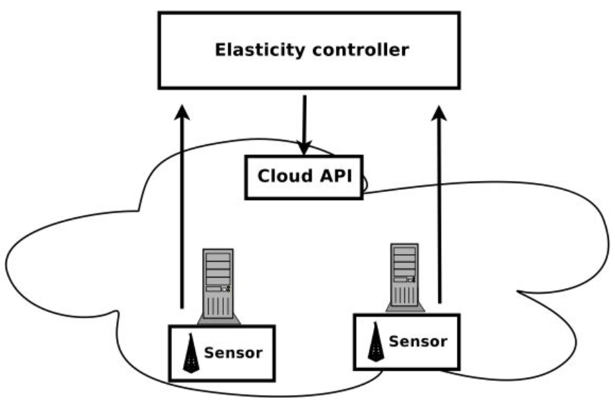
- Abstractly, an elasticity controller monitors allocated machines
- When overloaded, add load capability; When under used, reduce load capability
- Adding/reducing done by cloud framework (Cloud API), as directed by elasticity controller
- elasticity controller - approaches:
  - Per-tier controllers
    - Each application tier (e.g., web, logic, database) has its own controller.
    - Requires synchronization to avoid bottlenecks (e.g., one tier reducing resources while another still depends on them).
      - Tiers should only release resources when no interlock exists with another tier.
  - Single application-wide controller
    - Manages scaling decisions for all tiers together.
    - Allows developers to specify global scaling rules (e.g., scale the application logic tier when web requests exceed a threshold).
- elasticity controller - capabilities:
  - User takes monitoring offered, defines rules for when to take actions (models the application)
    - e.g. if CONDITION(s) then ACTION(s)
  - Monitoring, e.g.
    - resource usage
    - request sequence, looking for patterns to reconfigure for predicted load
    - server-level metrics like cost to benefit ratio
  - Triggering, e.g.
    - trigger on simple conditions, thresholds, on monitored instances, request stream
    - trigger on a schedule (simple prediction)
    - trigger on complex formula of many monitored instances (a model of overall service quality)
  - Actions, e.g.
    - Launch single instances, or identical instances, or modify existing instances
    - Execute sequence of launches or modifications according to a dependency graph or workflow
    - Execute programs that implement a more abstract action (launch and configure multi-tier service)
Server Scalability: Scale Load balancers
- Challenges: A single LB can become overloaded as the number of VMs increases, LB scalability should ideally grow at most O(p) (p = number of balanced VMs).
- Amazon Elastic Load Balancer (ELB): Provides VM-level load balancing but lacks built-in scalability mechanisms for LBs.
Network Scalability: Scaling the virtual network
- Router-based load balancing is an example of a network middlebox - Scaling middleboxes may need its own tier (especially if the function can be CPU intensive e.g., intrusion detection)
- Basic approach: split the flows
- “Load balancing the load balancers”
- Working with network switches & routers facilitates bandwidth allocation as well
- Dynamic Network Scaling
  - On-Demand Bandwidth Allocation: temporarily use unused bandwidth from other applications, or request additional bandwidth dynamically over existing links.
  - Network-Aware VM Provisioning: allocating bandwidth alongside VM provisioning
  - Network as a Service (NaaS): enables dynamic bandwidth allocation by e.g. Flow control, Distributed rate limiting, Network slicing; Statistical multiplexing to optimize network usage
Two-tier services: frontends (web) & backends (database)
PaaS Scalability: Containers and Databases
1. Containers
  - Multitenant containers allow different users’ components to run in the same container (better scalability) but require strong isolation (e.g., Java has security limitations).
  - Stateless components are preferred for easier scaling; Stateful components require additional management
2. Databases
  - distributed caching: improves performance by reducing database queries
  - NoSQL databases: Highly scalable and available (designed for cloud environments), uses eventual consistency
  - Database Clustering: Multiple SQL-compliant database nodes work together to distribute queries + replication to ensure high availability and fault tolerance
    - Scalability Challenges:
      - Maintaining consistency among multiple replicas can degrade performance.
      - Transactions lock data, causing conflicts when multiple queries try to update the same record.
      - High overhead due to synchronization across all nodes.
    - Middleware-Based Solutions:
      - Use proxy drivers to distribute queries across database replicas.
      - Handle request routing, load balancing, and replication consistency.

L02 - Private Cloud, OpenStack & P02 - OpenNebula

1. Private Cloud

Motivation
- heterogeneous machines, different user demands/workload - users {time, space} sharing machines
- limited resources - need for sophisticated VM placement (scheduling) stratagies
- security and privacy
- greater control
- want customization
  - e.g. current public cloud IaaS offerings are proprietary, i.e. do not allow experimentation etc.
- compliance
System Components
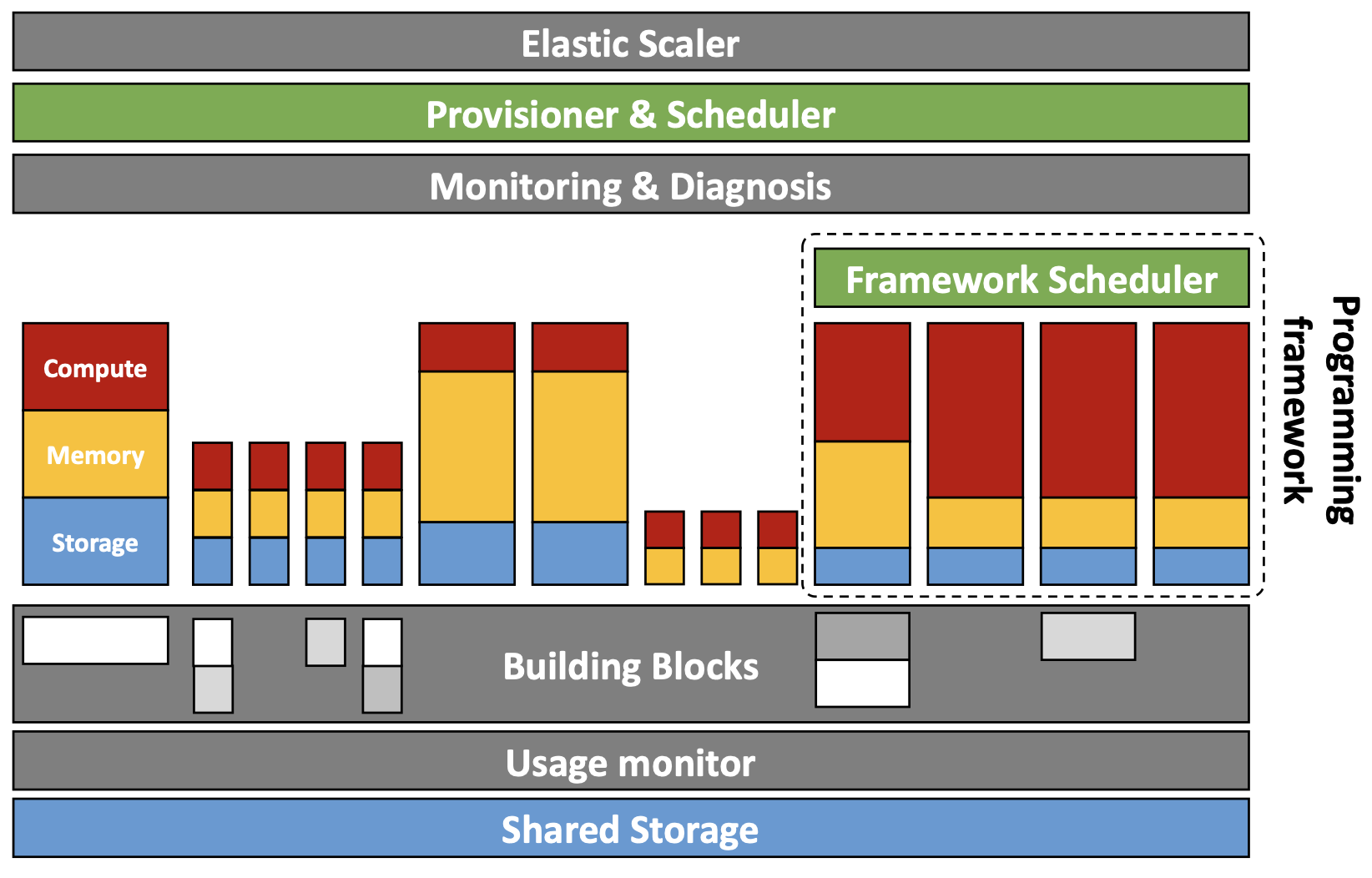
- Provisioner
  - Naive Provisioner: user requests for a specific number of cores, memory, storage (and other constraints / optional features), provisioner assigns users to machines: Bin-packing problem
  - Another Provisioner: pack cores, memory, and storage into a standard “set” and only allow the provision of a specific “set”
  - optimization: maybe migrate existing users for efficiency and capacity in resource allocation, but increase job runtimes
  - Provide a uniform and homogeneous view of virtualized resources
- Scheduler (resource allocation policies)
  - Goal 1: Prioritization
  - Goal 2: Oversubscription - Why: most users under-utilize resources
  - Goal 3: Workload constraints - e.g., Gang scheduling: must co-schedule distributed software that runs in lock-step
  - resource allocation policies should be flexible/configurable
- Encapsulation, isolation
  - solution: virtualization (do not solve all issues, e.g., performance interference)
- Fault Tolerance: replication; checkpointing, logging; geo-replication; etc.
- Provide Building Blocks (services) e.g., storage services, programming models and frameworks, load balancers, …
- Scaler + Monitor

2. OpemNebula

OpenNebula: virtual infrastructure manager + Haizea: resource lease manager
Design / Architecture: highly modular design with hooks
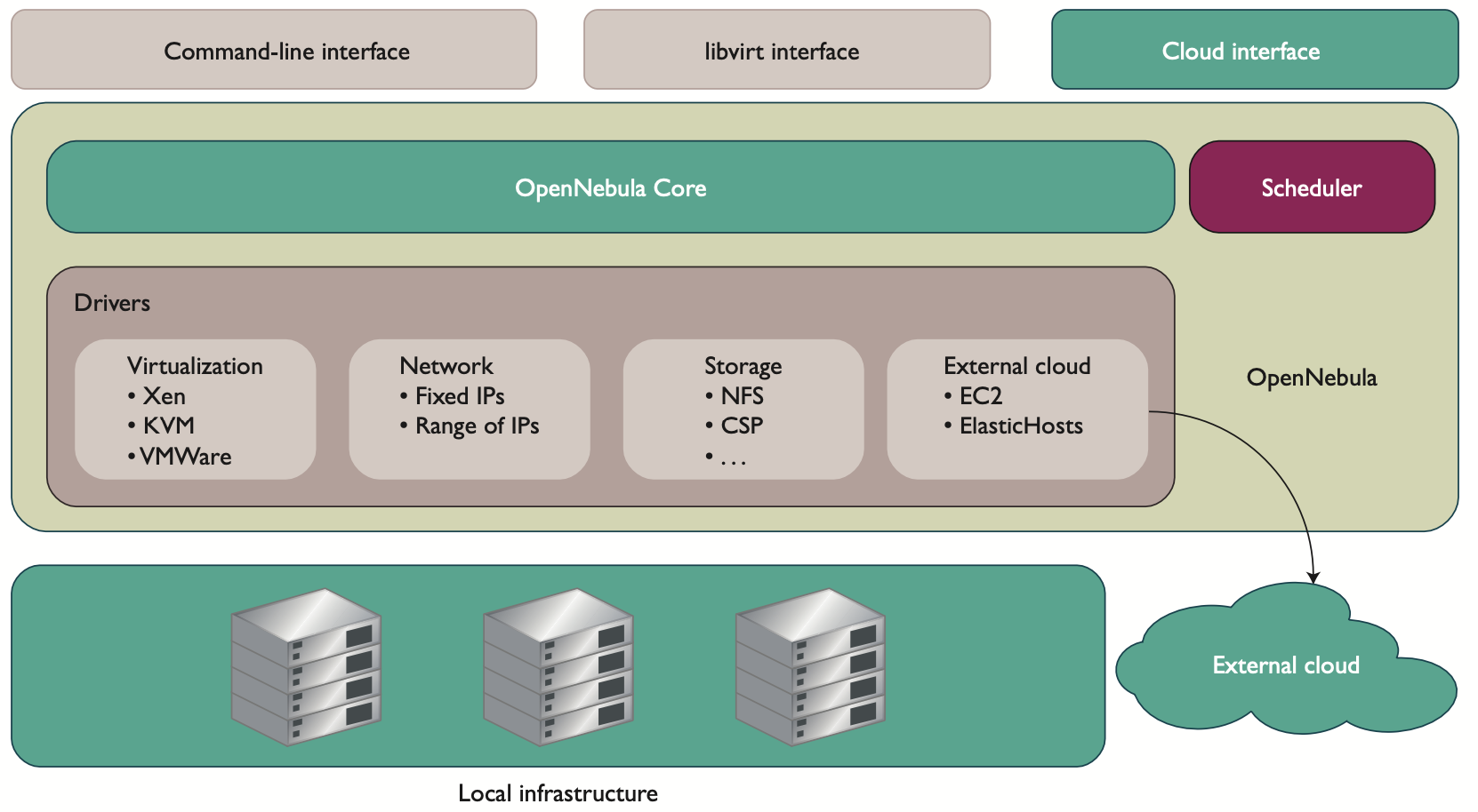
- Provides flexible and open architecture for building private/hybrid clouds
- OpenNebula Core:
  1. Manage Single VM lifecycle
    - image and storage technologies for preparing disk images for VMs
    - the network fabric for providing VMs with a virtual network environment
    - the underlying hypervisors for creating and controlling VMs
  2. service deployment
  3. delivery of context info to the VMs
- Virtualization, Network, Storage, External cloud drivers
- Scheduler
Haizea Lease Manager: use leases (advance reservation leases, best-effort leases, immediate leases)
- use VM for advance reservation lease:
  - resource preemption: suspending and resuming VM
  - Benefit: no need to vacate resources before an AR starts, improving efficiency and resource underutilization
  - Drawback: runtime overhead, preparation overhead

3. OpenStack

Cloud users and permissions
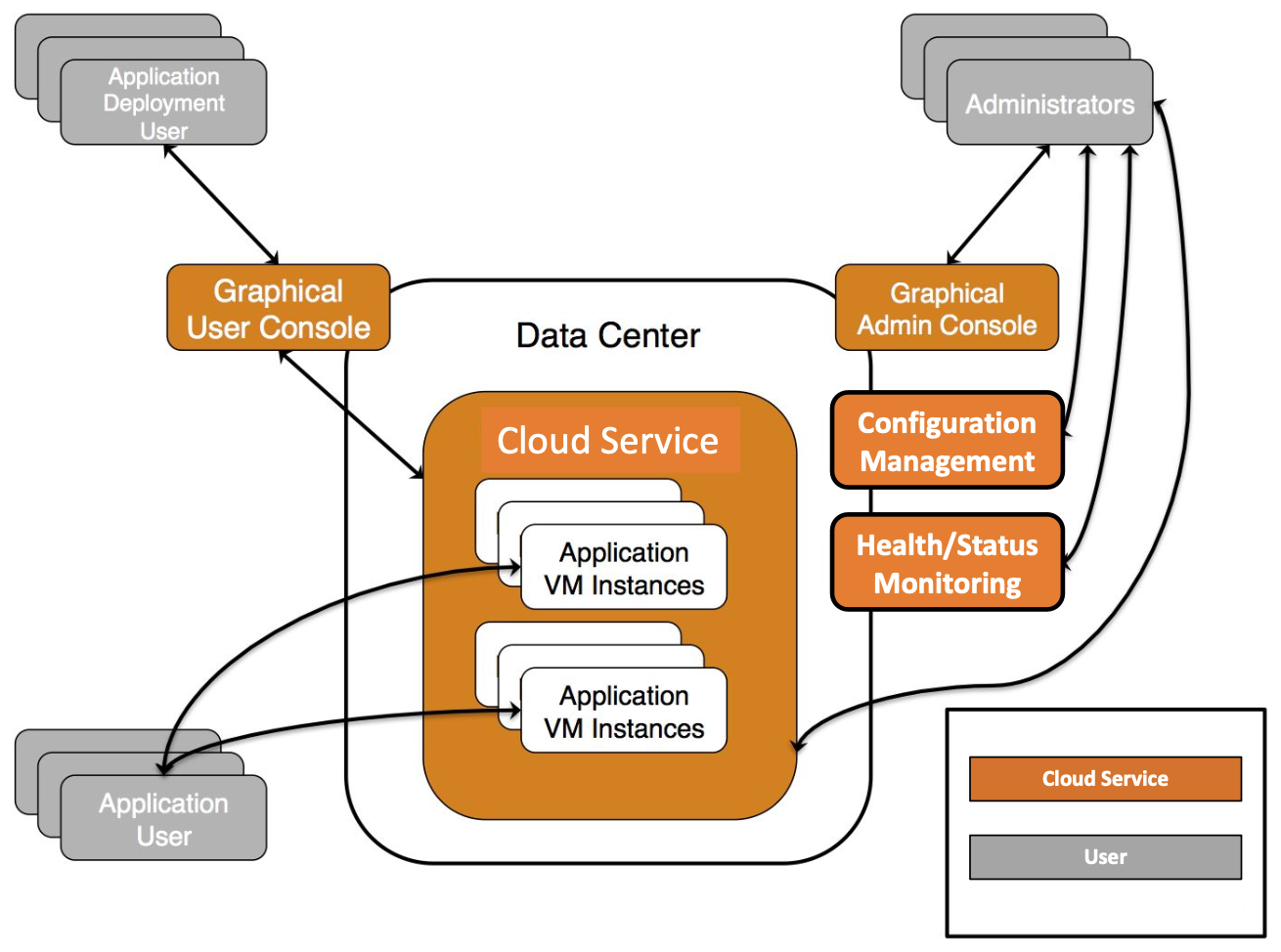
- application development/deployment user: sign up, credentialing, query system; modify data; provision and submit job
- Administrator: manage user accounts, monitor and manage resources
OpenStack Control: Managed pools of computing, storage, networking, etc, resources in a data center through a dashboard that gives administrators control and ability to provision resources

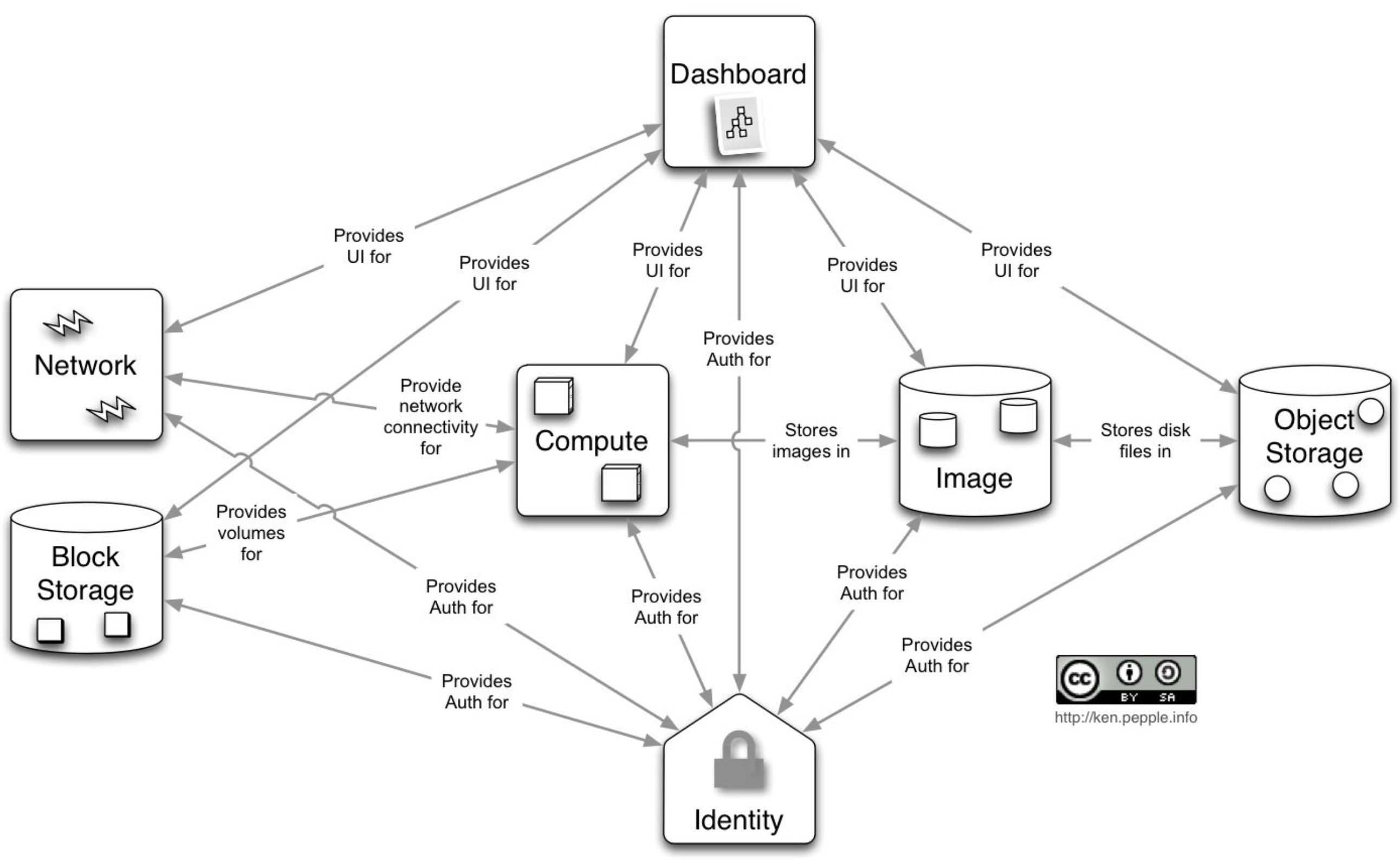
Architecture: independent parts named the OpenStack services

all authenticated through a common Identity service
communicate/interact through public APIs
Modular architecture (reuse existing infra)

Core services

Service	Codename
OpenStack Compute	Nova	(EC2) host and manage cloud computing systems
OpenStack Object Storage	Swift	(S3) Used for storing virtual machine images and data; Available from anywhere; REST API
OpenStack Block Storage	Cinder	(EBS) Used for adding additional persistent storage to a virtual machine (VM), access associated with a VM
OpenStack Networking	Neutron
OpenStack Identity	Keystone	authentication & authorization for other OpenStack services and users
OpenStack Image	Glance
OpenStack Telemetry	Celiometer	(Cloudwatch) gather, publish, and alarm on metrics and events
OpenStack Dashboard	Horizon

L03 - Encapsulating Computation

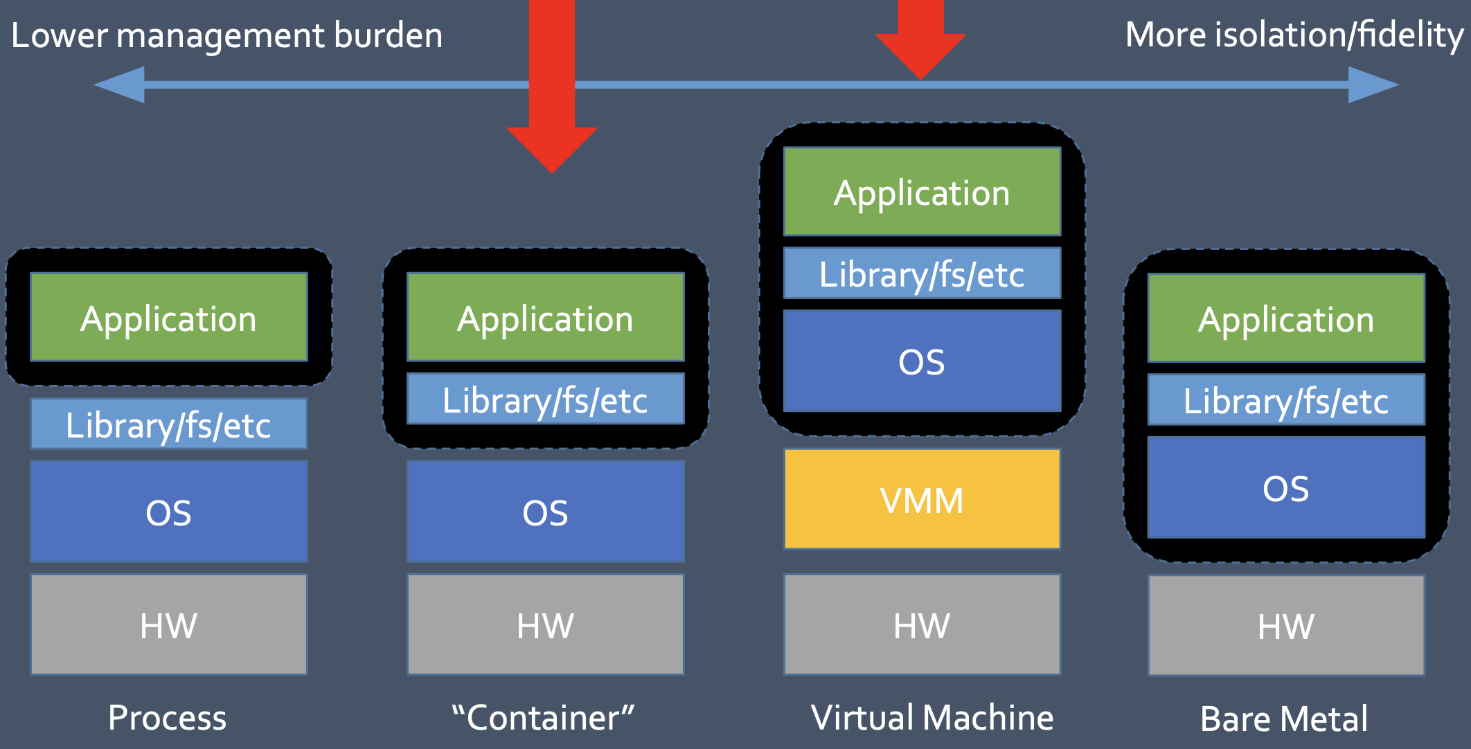
Options
- Bare Metal
- Pro: Good isolation, Software freedom, Best performance
- Con: Limits allocation granularity, Software management tricky (drivers, debugging OS)
- Process
  - Pro: Well-understood, Good performance, Debugging “easy”
  - Con: Performance isolation poor, Security questionable, Software freedom poor
- Containers
  - Pro: Decent software freedom, Good performance
  - Con: Possible security problems
- Virtual machines
  - Pro: Decent isolation properties, Good software freedom
  - Con: Performance overhead, Imperfect performance isolation
VM Techniques
- CPU Virtualization: Trap-and-emulate, paravirtualization
- …
VMM
- Type-I VMM vs. Type-II VMM
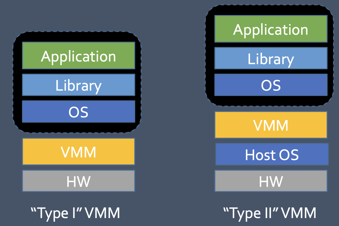
- Type I advantages: performance, smaller code base
- Type II advantages: convenience
Miscs from exam I review
- use case: paravirtualization > full hardware virtualization
  - When the guest OS’s device driver does many expensive (privileged), like reading and writing privileged control and status locations, there are many trap and emulation actions that the VMM must perform. With para-virtualization, the guest OS replaces a large chunk of its functions - the OS device driver for the virtual device - with a simple hypercall to the hypervisor specifying the device access with few (or zero) privileged operations and much less guest OS device driver work.
- use case: full hardware virtualization > para-virtualization
  - Allows the provider to determine and update their underlying OSes, including applying patches, without concern for customer software dependencies (e.g., particular OS and library versions).
  - Allows each customer to select their own software within their guest OSes, which may make the service more desirable.
  - Enhanced security. The provider may consider a VM-based approach to provide stronger security protections than the broader container interface to shared software.
  - Ability to run unmodified OSs within guest VMs. With paravirtualization, the guest OSs must be modified to interact properly with the hypervisor. With full hardware virtualization, the guest OSs need not be aware that they are not running on real hardware.
- use case: container > paravirtualizaiton
  - Any of launch speed, container image size, reduced patch requirements.
  - Generally speaking, containers can be started much more quickly, because less software needs to be executed to start them (container establishment vs. guest OS “boot”).
  - Container images also generally contain less software overall, making them smaller.
  - And, because they do not include a guest OS of their own, OS patches are not a requirement of each container image… though, independent updates of the underlying Linux OS can result in compatibility issues.
  - Containers have smaller footprint (because they share OS components and filesystem layers), hence achieving higher density
  - Container may have less performance overhead, because there is no need to go through two OS layers (guest and host).
  - Containers are more portable (do not depend on particular paravirtualized interface)
  - Containers are easier to maintain and manage, because they don’t require modification to the Operating System

L04 - Programming Models and Frameworks I: MapReduce and Spark

(& P04.1 MapReduce & P04.2 Spark)

1. High Performance Computing HPC

Perform simulations: Bulk Synchronous Processing (BSP) Model: iterate and propagate influence
- repeat: use previous time step values to update all mesh points in parallel, compute new values
Scaling in HPC: measures how performance changes when increasing processor count
1. Strong scaling: The same problem is solved faster using more processors.
2. Weak scaling: The problem size increases with the number of processors while execution time remains constant.
3. Key consideration: Problem size should be set to match the total available memory for efficient resource usage.
Characteristics:
- Runs on homogeneous machines
- High Cost of HPC Machines => need to maximizing utilization
- Resource sharing: space-sharing across physical clusters, meaning different workloads get allocated specific resources rather than dynamically sharing them.
- Requires low-level and hardware-specific optimizations
- Preferred for expert programmers following best practices
- Fault Tolerance via Checkpoint/Restart: require manual programmer intervention
  - Proto-elasticity: kill N-node job and reschedule a past checkpoint on M nodes
MPI (Message Passing Interface) Frameworks: Provides essential routines for parallel process management, including: Naming, addressing, membership; Messaging, synchronization (barriers); Math and physics libraries.
Grid Computing: an extension of High-Performance Computing (HPC) by utilizing distributed computing resources
- replace traditional supercomputers with clusters of smaller, cheaper machines.
- less specified, easier to use, but less efficient
- geographical sharing resources (collaboration between multiple institutions): heterogeous workflow
- Job scheduling: use a queue, and schedule with available resources in the cluster
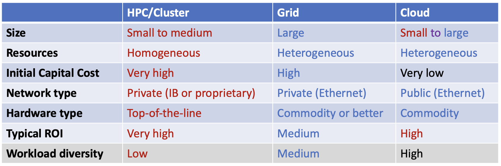
Programming models - comparison:

2. MapReduce

Data parallel framework for processing Big Data on large commodity hardware
stratages
- Parallelism: Break down jobs into distributed independent tasks to exploit parallelism
- Scheduling: Consider data-locality and variations in overall system workloads for scheduling
- Fault Tolerance: Transparently tolerate data and task failures

=> Slide Page 20 onwards

Advantage
- Independent
  - Easy to program when there are no computational dependencies
  - No communication between functions, no synchronization
  - Fault tolerance, simply restart function
  - Speculative execution when there are stragglers: launch another instance of a slow-running task on a different node to mitigate the impact of slow shuffles
- Parallel
  - High performance when the application is embarrassingly parallel

3. DryadLINQ

4. Spark

Lazy evaluation. Advantage: batching/combining of operations (data transformations), which allows multiple operations to be computed in one pass (minimize the number of data passes), and can avoid unnecessary reads, writes, and GC

5. MapReduce vs. Spark

	MapReduce	Spark
	(-) MapReduce has a high overhead for disk I/O for input, intermediate, and output	(+)
	(-) Limited semantics with Map followed by Reduce	(+) Spark oﬀers various functions with a generalized DAG

L05 - Programming Models and Frameworks II: Iterative Computation

1. MapReduce, Spark and Parameter Server for ML

Machine Learning Stages
1. Data collection (Logistics, cleaning, …): Done mostly away from machine learning data center, then aggregated
2. Model selection: Done offline from collection/engineering/training/inference
3. Data engineering (Extract, transform, …): Multiple data passes (Map/Reduces), large data reduction, more cleaning
4. Model training: iterate many times (many data passes)
5. Model inferencing: For one input, apply model and return one predicted output (no data passes)
ML model training via MapReduce: inefficient
- Approach:
  1. each map task processes a subset of input data and computes parameter updates
  2. updates are then shuffled (redistributed) to reducer tasks, which aggregate them into a single output
  3. aggregated parameters are collected by the driver and broadcast for use in subsequent iterations
- Overhead from task initialization: If Hadoop, each map and each reduce task are Java VM launch
- Inefficient iterative process: Iteration is in external scripts repeating Hadoop invocations
- Low compute per data item, leading to the fixed overhead becomeing high
- Mapper: Redundent updates and Reduced data shuffle: No need to issue parameter update per data item; could pre-combine updates for same parameter in memory of each map, so reduced data shuffle, and do a single set of parameter updates per map
- Reducer: Simple aggregation: add updates for each parameter, cost is at communication through file system
- Overall: it may scale great, but has heavy network traffic and significant task overhead
ML model training via Spark: better
- Cache in memory
- Driver collect & broadcast for parameters
- Combine map transformations to try for one shuffle per iteration
- retain one VM for all tasks across all iterations, so less overhead
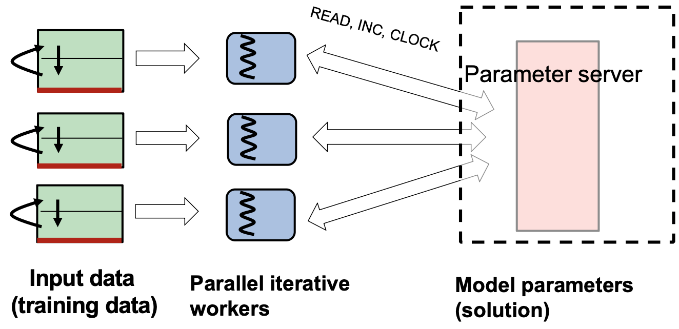
Parameter Server
- Shared Memory Model for Parameters: maintains a centralized, logically shared memory space for the model parameters
- Atomic Updates for Parameters: the worker can directly push or pull an incremental change to/from the parameter server
- Benefits: Reduced Data Transmission, Lower Task Overhead, Simpler (No) Data Repartitioning, Scales well
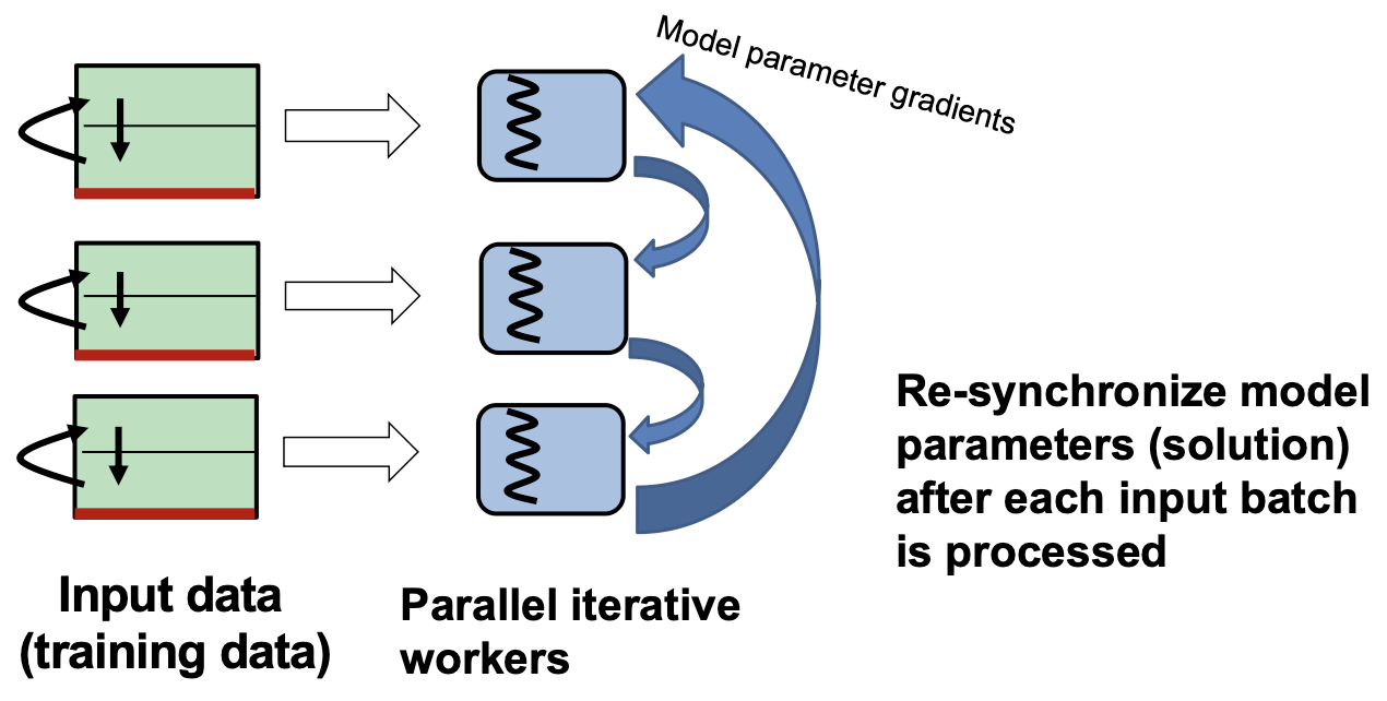
- Allreduce operation: synchronize updates efficiently without relying on a centralized parameter server

P05 - Parameter Server

1. Introduction and Motivation

Need for distributed processing: training data size (TB-PB), parameters (billions-trillions), computational and communication demands
Challenges with Shared Parameters
- Network Bandwidth: Frequent access to shared parameters by all workers
- Sequential Algorithm Constraints: Many machine learning algorithms are inherently sequential, which creates bottlenecks when parallelized.
- Memory and Access Constraints: No single machine can hold the entire parameter set in memory
Distributed machine learning algorithm: Each worker only caches/processes the subnet (“working set”) of parameters it needs (e.g., 7.8% with 100 workers, dropping further with more nodes)

2. Parameter Server

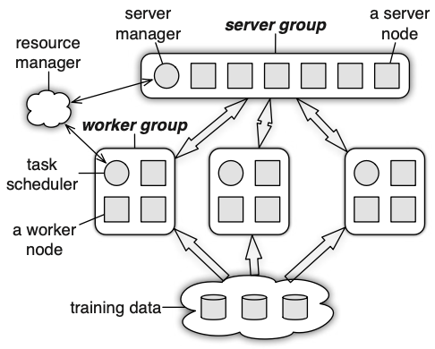
Overall System Architecture
- A single parameter server instance can run multiple algorithms simultaneously.
- Parameter Namespaces: Support isolation between different worker groups.
  - Multiple groups can share the same namespace to boost parallelization or to allow simultaneous model querying and updating
- Node Groups:
  - Server Group:
    - Contains server nodes that maintain partitions of the globally shared parameters.
    - Server nodes communicate to replicate or migrate parameters for enhanced reliability and scalability.
    - A dedicated server manager maintains metadata (e.g., node liveness and partition assignments).
  - Worker Groups:
    - Each worker group runs an independent application.
    - Workers locally store portions of training data to compute local statistics (such as gradients).
    - Workers communicate exclusively with server nodes - not with each other.
    - Each group is managed by a scheduler that assigns tasks, monitors progress, and reschedules unfinished tasks when the number of workers changes
Key Features
- Efficient Communication:
  - asynchronous operation: minimize blocking of computation
  - batch updates: exploits the structured nature of ML parameters (vectors, matrices, tensors) and reduces overhead
- Elastic Scalability: Supports dynamic addition of nodes without requiring system restarts
- Fault Tolerance and Durability:
  - Implements rapid recovery through live replication and the use of vector clocks
  - Supports continuous operation despite non-catastrophic failures
- Flexible Consistency Models
- Ease of Use: Represents shared parameters as (key, value) vectors
System design
- Model representation: a set of (key, value) vectors
- Communication (data transfer): Range Push and Pull: specify a key range $R$ to limit communication to only a subset of the parameters
- Server capability: the server not only aggregates data, but can also execute custom user-defined functions
- Task issuance and execution: asynchronous, dependency can be enforced to serialize tasks
  - ML workflow is often tolerant of asynchronous updates because ML is an iterative approximation converging to the optimum
- Flexible consistency: allow the designer to define the consistency model: sequential consistency, eventual consistency, $\tau$ bounded delay
- Fine-grained control of data consistency: allow user-defined filters to selectively synchronize individual (key, value) pairs, enabling the algorithm to push only the most relevant or significantly changed parameters
Implementation details
- Vector Clock: to track the version or timestamp for each (key, value) pair across all nodes, providing aggregation tracking, duplicate detection, consistency and recovery
  - Optimization: Range compression
- Messages: a list of (key, value) pairs over a key range R - Range-based communication
  - Optimization: key caching, value compression
- Consistent Hashing
- Replication: Each server node stores replicas of the key ranges of its k counter-clockwise neighbors (acting as slaves), update on the master is synchronously pushed to its slave nodes
  - Optimization: Only the aggregated result is replicated, reducing network bandwidth usage significantly
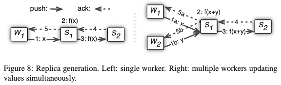
  - With k replication typically small and n num_of_workers being large, replication overhead is minimized while still maintaining consistency
- Server Group Management: dynamic scaling & fault tolerance
  - node join: two-stage data fetch
  - node leave (e.g. failure): detect by heartbeat
- Worker Group Management: dynamic adjustment by task scheduler

L06 - Key-Value Stores & P06 - FAWN

1. Key-Value Stores

Plain text keys vs. Hash keys
- Plain text keys provide: Potential for range queries, Sorting
- Hash keys provide: Potentially smaller/fixed-size keys, Load balancing
Motivation: KV-pair is usually small, so overhead matters. Want High throughput (performance) / low latency (cost)
Workload: IO intensive, require random access over large datasets, parallel, high load requires large clusters, size of object is small
benefit over row-based data store:
- suitable for the workload of caching or object stores
- High throughput / Low overhead / scalability
- Low latency / fast lookup
- No need for schema / structure (enabling low overhead)

2. Memcached: in-memory KV cache

use case: small objects (90% keys < 31 bytes), high QPS (10’ of millions), read-mostly workloads
Design:
- index data structure: hash table with chaining
- Slab-based Memory Allocation: avoid allocation overhead, reduce fragmentation, re-use memory
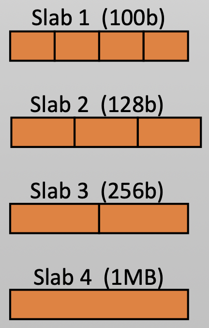
- LRU: a doubly-linked list for each slab
Problem:
- Single-node scalability and performance, poor use of multiple threads
- space overhead: 56-byte header per object (~50% overhead), poor hash table occupancy
- Improvement: MemC3: use optimistic cuckoo hashing: higher concurrency (single-writer/multi-reader), better memory efficiency
Multi-node Memcached Clusters: can have a request director/load balancer

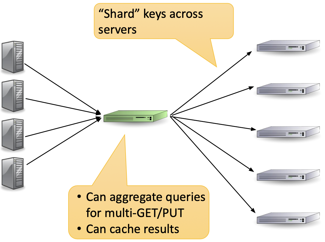
3. FAWN-DS: on-flash KV storage

Flash storage performance:
- Read/write performance between DRAM and Disk
- Fast random reads, slower random writes
- overwrite existing data (need first erasing) is inefficient
Design
1. log-structured writes 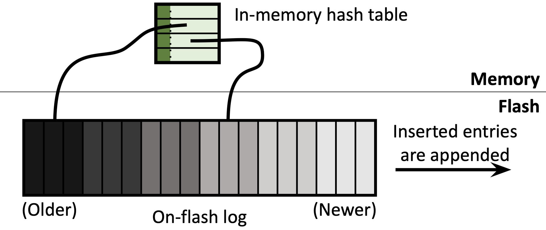: random reads, sequential writes
2. Minimize I/O: Low prob. of multiple flash reads
3. Memory efficient: 12 bytes per index entry
GET() operation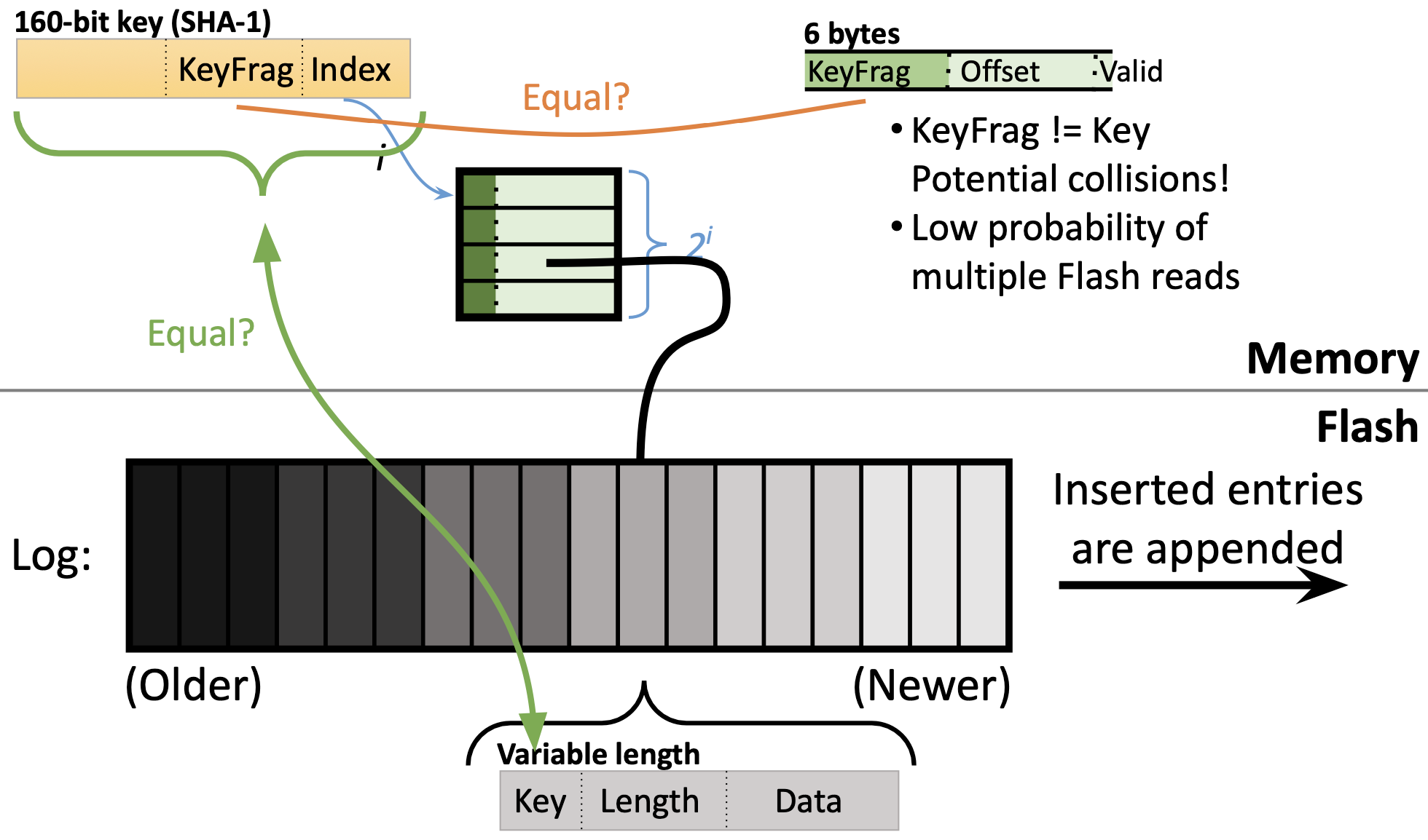
- $160$ -bit key
- $i$ index bits: used to select a bucket from the total $2^i$ hash buckets
- each bucket have 6 bytes: 15 bit KeyFrag, 1 valid bit, and 4-byte pointer to log location
- $15$ bits key fragment: use to compare value in hash bucket. If KeyFrag do not match, use hash chaining for next in hash table
- Reads the record from flash memory (the log), which contains the full key. If key does not match, do second fetching (1 over 32,768 chance)
API: operation: store, lookup, delete; maintenance: split, merge, compact
- Concurrent Maintenance and Operation: maintenance operation runs until it reaches the end of the log, then briefly locks the datastore for updating.
Failure Recovery / Reconstruct: use the on-flash log to reconstruct the index + periodic checkpoint for faster recovery

4. FAWN-KV: distributed KV storage

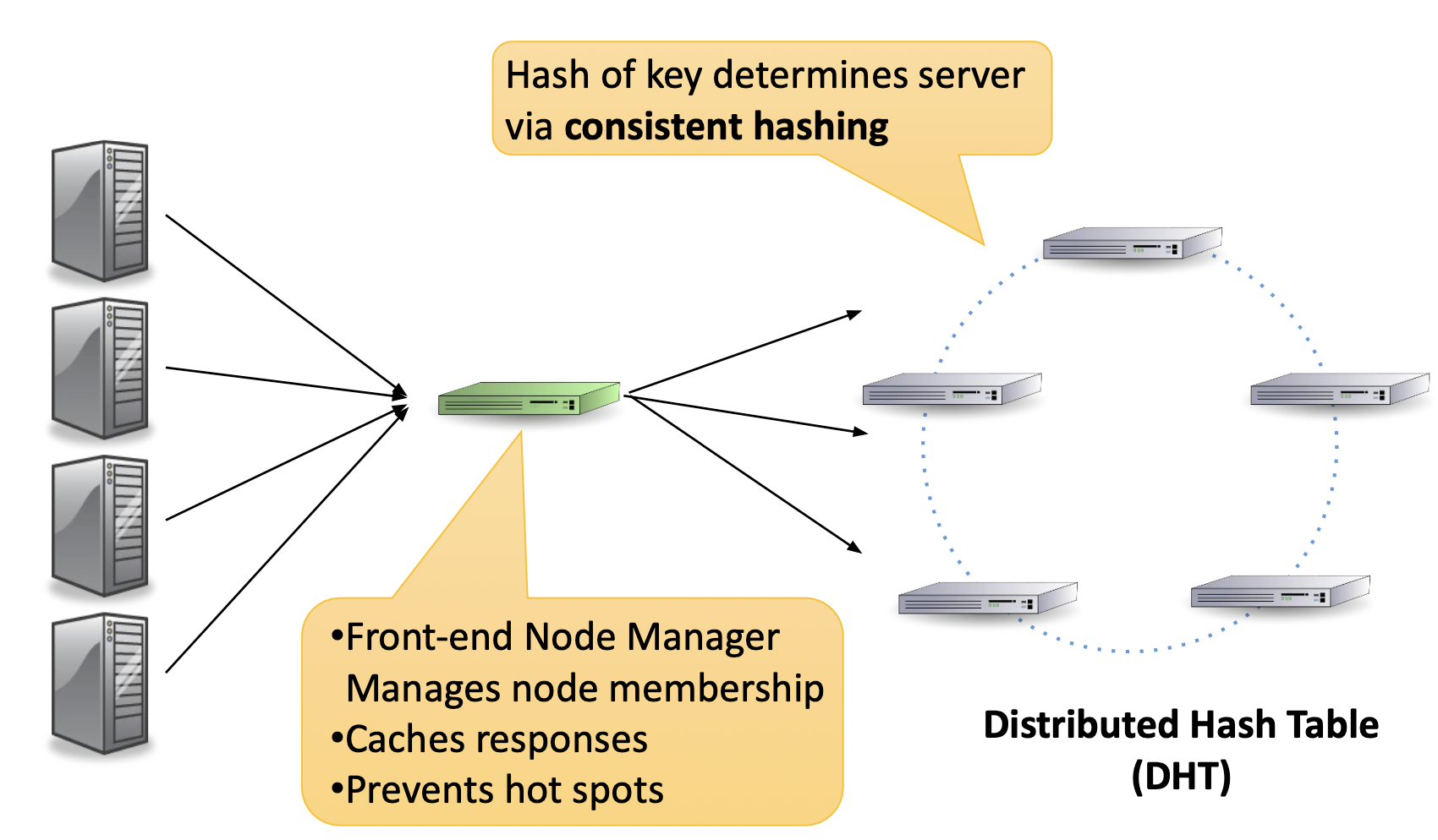
Front-end
- Advantages:
  - Ability to cache hot keys
  - Ability to aggregate queries and batch them to the storage nodes
  - Ability to load balance requests among replicas
- Disadvantages:
  - Complexity (e.g., clients need to know about the storage nodes)
  - Additional point(s) of failure
  - Need for cache coherence (when using multiple front-ends that are caching keys)
DHT: consistent hashing
transfer key range operation: background operation, concurrent with inserts, minimizes locking
Chain replication
- Three copies of data on successive nodes in ring (head-middle-tail)
- Insert at head, read from tail
- Strong Consistency: Don’t return to client until all replicas have a copy
- Every node is part of three chains
Load Balancing (handle hotspots): use a popularity cache on the front-end node

L07 - Edge Computing & P07 - Cloudlet

Need for edge computing: mobile apps need processing capacity of clouds, but with strict timing requirements
- offload: computation, (CPU, networks, storage)
- Energy limits on mobiles (limited by thermals)
Why Edge Computing better than Clouds
- Lower Response Time (latency), also avoid variation in latency to access the cloud
- Lower energy consumption on mobile device
- high bandwidth to upload data (such as video)
- Cost of storing unneeded data, filter on the edge and store what’s relevant
- Privacy, some data should not be uploaded to the cloud
Cloudlet definition
- use case: a mobile user exploits virtual machine (VM) technology to rapidly instantiate customized service software on a nearby cloudlet and then uses that service over a wireless LAN, the mobile device typically functions as a thin client, with all significant computation occurring in the nearby cloudlet
- A cloudlet is a trusted, resource-rich computer or cluster of computers that’s well-connected to the Internet and available for use by nearby mobile devices
- Cloudlet-based, resource-rich, mobile computing
- Provide: low-latency, one-hop, high-bandwidth wireless access to cloudlet for mobile client
Cloudlet design & features
- Local cloud infrastructure over LAN/WLAN - exploit proximity to users, provide high bandwidth, low latency relative to cloud; need for discovery
- provide IaaS - dynamic, on-use provisioning at edge
- decentralized, incremental deployment - like WiFi
- only soft state - keeps management overhead low
- May need to migrate services between cloudlets as user moves

Approaches to deliver VM state to cloudlet

VM migration

VM vs. Container	VM	Container
Launch time	Slow	Fast - no booting
Transfer/migrate time	Slow	Fast
Memory footprint	large	small
	General - OS, kernel dependency	not general
isolation		less
(Live) Migration	Yes	Hard - process state with the kernel, etc.

VM Synthesis: dividing a custom VM into Base VM and VM overlay - rapid provisioning of cloudlet resources
- Base VM: Vanilla OS that contains kernel and basic libraries
- VM Overlay: compressed diff between custom, standard VM
- Optimization:
  - minimize VM overlay size: deduplication, reduce semantic gap by including only the state that actually matters to the guest OS
  - accelerate VM synthesis: pipeline, early start

P08 - Hadoop Distributed File System (HDFS)

1. Definition, Introduction, and misc information

partitioning of data and computation across many (thousands) of hosts, and executing application computations in parallel close to their data
HDFS stores file system metadata and application data separately
The DataNodes in HDFS do not use data protection mechanisms such as RAID to make the data durable. Instead, like GFS, the file content is replicated on multiple DataNodes for reliability.

2. Architecture

NameNode: maintains the namespace tree and the mapping of file blocks to DataNodes
- Namespace is a hierarchy of files and directories; Files and directories are represented on the NameNode by inodes with metadata (e.g. permissions, modification and access times, namespace and disk space quotas); The file content is split into large blocks (typically 128 megabytes) and each block is independently replicated

L08 - Cloud Storage

“Object” (or “blob”) store - arbitrary-sized “files” with simplified interface
- Usually limited interface and semantics, e.g., CRUD API: Create, Read (get), Update (put), Delete, No open/close, rename, links, locks, etc - simplifies scaling, code paths, caching, use other space-saving encodings, etc.
Block stores (virtual disks) - separate but attachable to any VM instance
- Virtual disk looks to guest OS just like real disk
- often implemented as files
- Thin provisioning (“over-provisioning”)
“Local disk” as part of VM instance - exists for lifetime of instance
- visible only to the instance it comes with, cannot be attached to a different VM instance
“Traditional” distributed FS
Union FS

L09 - Tail Latency

(& P09 - The Tail at Scale)

1. Introduction

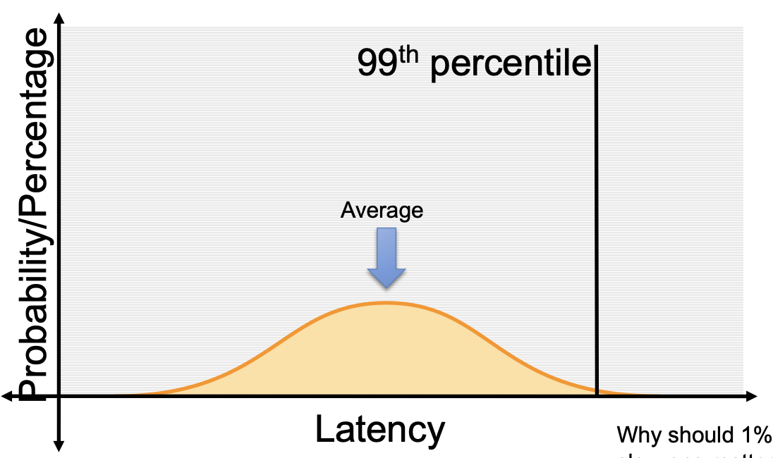
Scenario 1: Even rare performance hiccups affect a significant fraction of all requests in large-scale distributed systems
1. User: Very slow responses make for angry users
2. Big jobs / large fan-out: Big (parallel) jobs often wait for their last task to finish, so runtime is the max task time rather than the average
Scenario 2: Component-level variability amplified by scale
- $P(\text{acceptable service latency}) = P(\text{acceptable latency on a single sub-operation})^n$
Scenario 3: Eliminating all sources of latency variability in large-scale systems is impractical, especially in shared environments
Aim: to keep the tail of latency distribution short, “latency tail-tolerant”, “tail-tolerant”
- better to have them all be a little slow, than to have some very slow
- tail-tolerant software techniques form a predictable whole out of less-predictable parts

2. Service/response time varies for many reasons

Shared resources (e.g. CPU cores, processor caches, memory bandwidth) & Global resource sharing (e.g. network switches and shared file systems) & Shared infrastructure (e.g. a VM sharing CPU with other compute-bound VMs, “serverless” computing)
Background daemons & Maintenance activities (e.g. periodic garbage collection, data reconstruction in distributed file systems): when scheduled, can generate hiccups
Queueing: amplify the variability
Caching (unless the entire working set can reside in a cache)
Hardware: power limits, (storage) garbage collection, energy management (power-saving modes)

3. Reduce component variability

Prioritize / Differentiate service classes and higher-level queueing
- e.g. prefer scheduling requests for which a user is waiting over non-interactive requests
- e.g., do the stuff that is being waited for first (before background stuff)
- e.g., do the stuff that is “falling behind” first
Reduce head-of-line blocking: break long-running requests into a sequence of smaller requests to allow interleaving of the execution of other short-running requests, to avoid a small number of very computationally expensive queries from adding substantial latency to a large number of concurrent cheaper queries
Manage background activities and synchronized disruption
- throttling, breaking down heavyweight operations into smaller operations, and trigger such operations at times of lower overall load
- for large fan-out services (parallel), synchronize the background activity across many different machines. This synchronization enforces a brief burst of activity on each machine simultaneously, slowing only those interactive requests being handled during the brief period of background activity.

4. Tail-tolerant techniques

Within Request Short-Term Adaptions: effective only when the cause of variability does not simultaneously affect multiple request replicas
- Hedged requests: issue the same request to multiple replicas; use the first response and cancel others
  - to avoid adding unacceptable additional load (2x): e.g. defer sending a secondary request until the first request exceeds the 95th-percentile latency for similar requests (5%)
- Tied requests: to address variations introduced by queuing. Simultaneously enqueue requests on multiple servers with cross-server status updates
  - the client send the request to two different servers, each tagged with the identity of the other server (“tied”) => When a request begins execution, it sends a cancellation message to its counterpart. The corresponding request, if still enqueued in the other server, can be aborted or deprioritized
  - requests should be idempodent to avoid double-execution
- Least-loaded server probing: probe remote queues and send requests to the least-loaded server (less effective than tied requests because (1) load levels can change between probe and request time; (2) request service times can be difficult to estimate due to underlying system and hardware variability; and (3) clients can create temporary hot spots by all clients picking the same (least-loaded) server at the same time)
- Application in complex coding schemes: Send requests to the primary server and, after delays, issue requests to replicas, to reconstruct data via tied requests
  - The Distributed Shortest-Positioning Time First system: forward requests to replicas if the initial server does not have it in its cache
Cross-Request Long-Term Adaptions: reducing latency variability caused by coarser-grain phenomena (e.g. service-time variations and load imbalance: the performance of the underlying machines is neither uniform nor constant over time, outliers in the assignment of items to partitions can cause data-induced load imbalance)
- Micro-partitions: generate many more partitions than there are machines in the service, then do dynamic assignment and load balancing of these partitions to particular machines. Load balancing is then a matter of moving responsibility for one of these small partitions from one machine to another
- Selective replication: Create additional replicas of items that are likely to cause load imbalance. Load-balancing systems can then use the additional replicas to spread the load of these hot micro-partitions across multiple machines
- Latency-induced probation: exclude a particularly slow machine, or putting it on probation. However, continue to issue shadow requests to these excluded servers, collecting statistics on their latency so they can be reincorporated into the service when the problem abates

5. Tail-tolerant techniques in Large Information Retrieval (IR) Systems

Speed is a critical quality metric, prioritizing fast, “good-enough” results over slow, perfect ones.
Good Enough Results: serve slightly incomplete results once a sufficient fraction of servers responds, avoiding delays caused by slow servers. e.g. Nonessential subsystems (e.g., ads, spelling correction) are skipped if they do not respond in time
Canary Requests
- to prevent widespread correlated crashes in systems with very high fan-out: a particular request exercises an untested code path, causing crashes or extremely long delays on thousands of servers simultaneously
- Root servers first send requests to one or two “canary” servers to test for crashes or long delays, flag dangerous requests before querying all servers
- Adds minimal latency while improving system robustness against errors or denial-of-service attacks

6. Other factors: Mutation and Hardware

Mutations of system state in Latency-Critical Systems: are less impacted by latency variability due to:
- Smaller scale of latency-critical updates
- Updates often performed off the critical path after user response
- Many systems can tolerate inconsistent update models for (inherently more latency-tolerant) mutations
- Consistent updates use quorum-based algorithms (e.g., Paxos), which are tail-tolerant as they only require consensus among a few replicas
Hardware trends: Increased variability due to aggressive power optimizations and device heterogeneity from fabrication challenges => will require more reliance on software techniques to tolerate latency variability

L10 - Data lakes, warehouses, Lakehouse

1. requirements of data solutions

Reliability - Data should not be lost or corrupted.
Scalability - Handle large datasets and high-concurrency workloads.
Performance - Querying, modifying, and processing data fast and efficient.
Governance - Proper security, access control, and auditing in place.
Flexibility - Data should support both structured and unstructured formats.

2. Data Lakes

Definition: Scalable, cost-effective, and flexible repository for storing structured, semi-structured, and unstructured data
- Enables data processing with nearly any tool desired: can read/write data directly from/to data lakes, with little-to-no overhead
Design:
1. Big shared collection of files/objects, e.g.Objects/blobs in clouds
2. Indexes: for efficient data retrieval
3. Catalog of metadata: to discover, understand, and manage data (identities+attributes of each file/object): Usually some sort of DBMS
Advantages:
1. Scalable and cost-effective - Store massive amounts of data at a low cost.
2. Flexible data storage - Support structured, semi-structured, and unstructured data.
3. Decoupled storage and compute - Enable multiple processing engines to analyze the same data.
4. Supports advanced analytics - Ideal for big data, AI/ML, and real-time processing.
Disadvantages:
1. Lack of ACID transactions - Hard to enforce consistency, updates, and deletes.
2. Slow query performance - Requires full scans, leading to high latency and costs.
3. Metadata management challenges - Handling large numbers of files can reduce efficiency.
4. Complex security and governance - Fine-grained access control is harder to implement.

3. Data Warehouses

Definition:
1. System for collecting and managing data from varied sources to provide meaningful business insights (BIs).
2. System to support query and analysis on historical data derived from transaction data. It usually includes data from other sources. i.e. Separate analysis workload from transaction workload.
3. Generlly performs OLAP workload
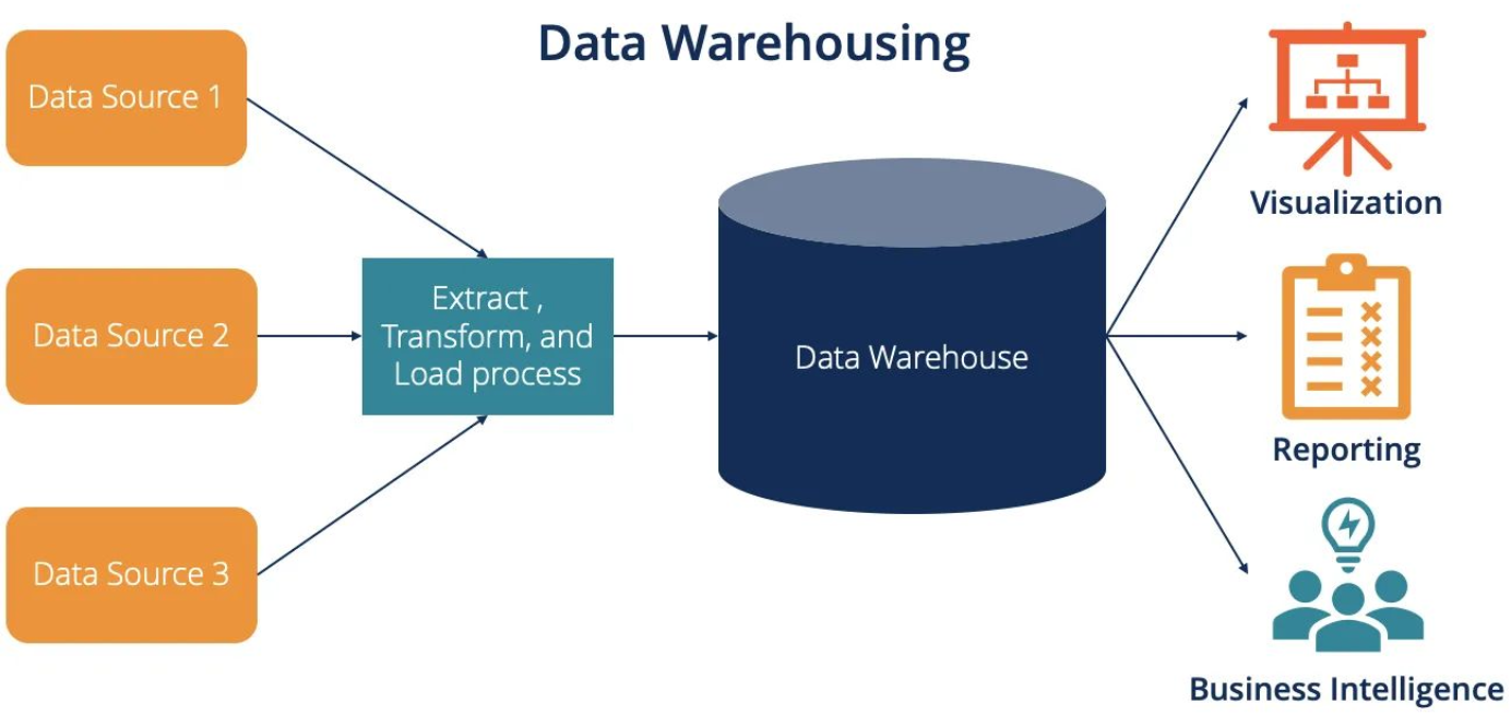
Cloud Data Warehouses e.g. Amazon Redshift

4. Lakehouse

(See section P10 first)

Metadata Layer: Delta Lake: Data Management and Governance
- An ACID table storage layer over cloud object stores
- Intercepts reads & writes to update a centralized transaction log
- This approach offers: Transaction log, Scalable Metadata Handling (Fast metadata operations), Schema Enforcement and Evolution, Audit logs, Time travel, Zero cost clones
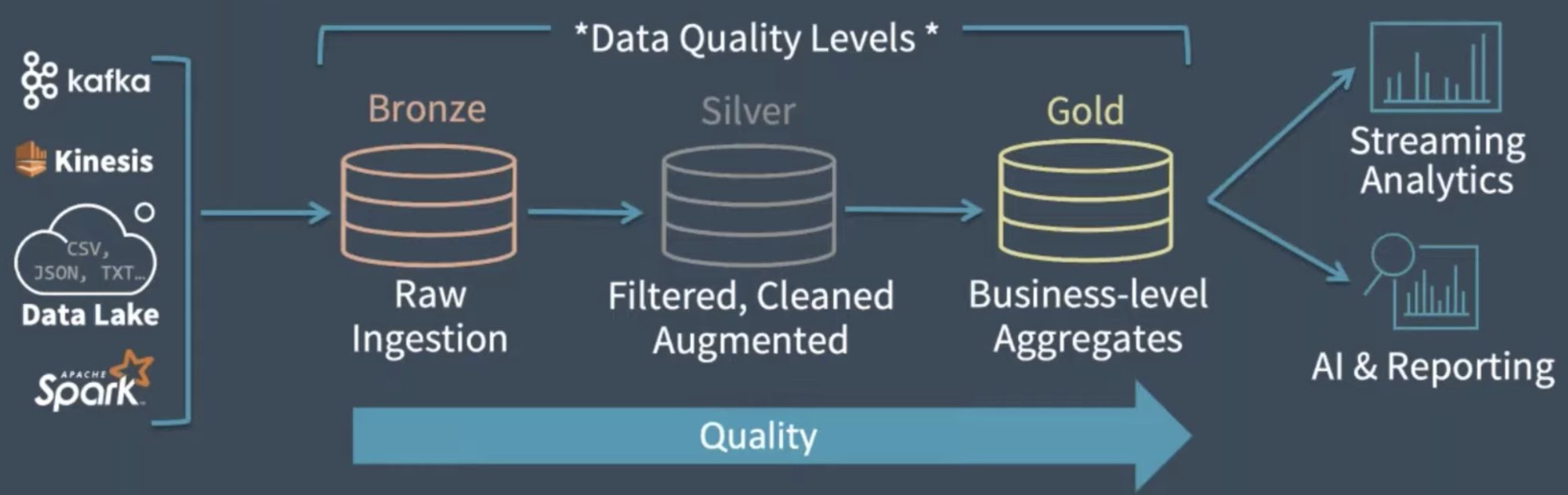
- Multiple Data Quality Levels: Bronze, Silver, Gold:

P10 - Lakehouse

1. Data Warehouse - history

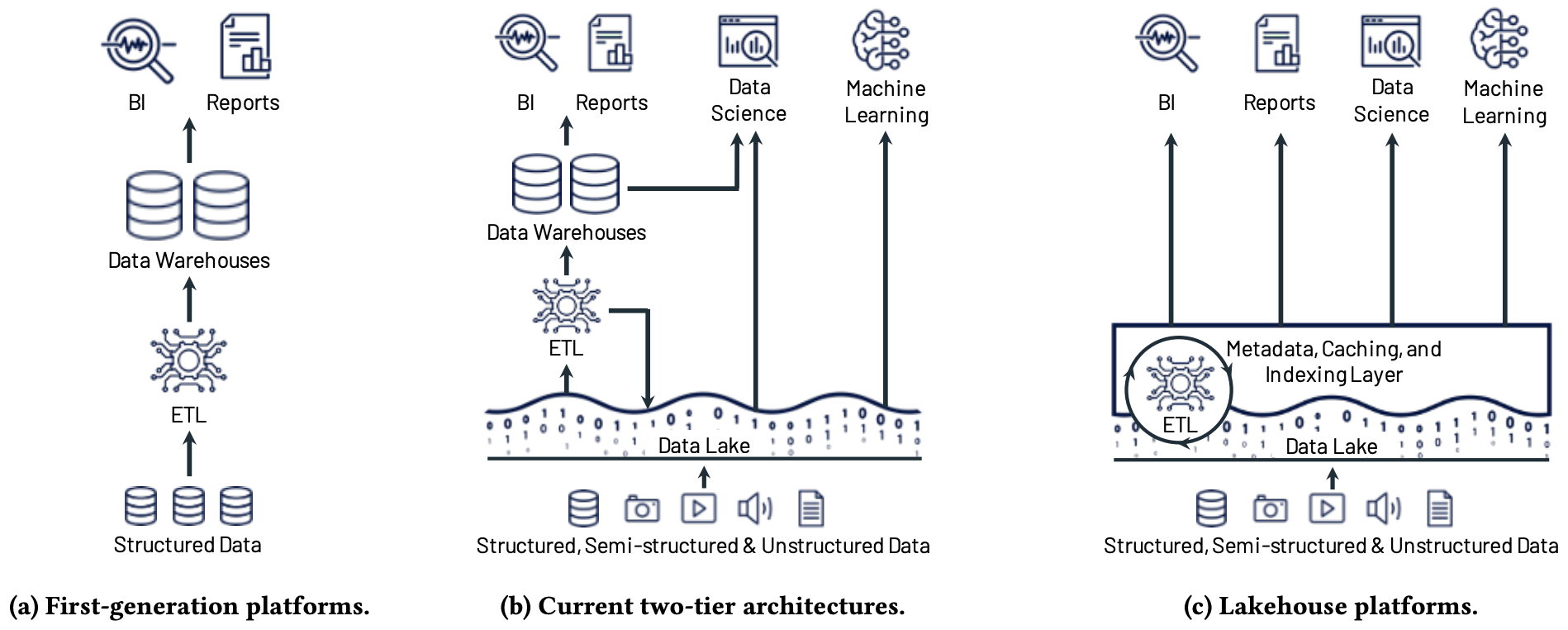
first generation data analytics platforms: Data in warehouses for decision support and business intelligence (BI). Data written with schema-on-write, ensuring that the data model was optimized for downstream BI consumption.
- data flow: operational data systems =(ETL)=> warehouse
- Challenges:
  1. Coupled Compute & Storage: On-premise appliances required provisioning for peak loads, leading to high costs
  2. Growing & Unstructured Data: datasets grows rapidly, and data warehouses could not store and query unstructured datasets, e.g., video, audio, and text documents
second generation data analhytics platforms: data lakes: low-cost storage systems with a file API that hold data in generic and usually open file formats
- schema-on-read architecture: enable store any data in open file format at low cost
- shifted data quality/governance issues downstream
- For BI workloads: ETL process moved a subset of data to downstream data warehouses for BI
  - data lakes =(ETL)=> warehouse [for BI]
- For advanced analytics or machine learning workloads: Open formats enabled direct access for analytics
  - data lakes =(direct read)=> machine learning analytics
current two-tier architecture: cloud data lakes (e.g. AWS S3) + warehouse
- two-tier architecture: separate storage and compute
  - cloud data lakes: benefits: durability, geo-replication, extremely low cost with the possibility of even cheaper archival storage, etc.
  - downstream data warehouse (usually SQL-based data warehouse)
  - data flow: operational data systems =(ETL)=> data lakes =(ETL)=> warehouse
- Challenges:
  1. Data Quality & Reliability:
    - Two-tier architecture adds complexity, delays, inconsistencies, and failure risks.
    - ETL introduces failure risks and data quality issues: e.g., due to differences in data types, SQL dialects, and schemas between lakes and warehouses.
    - Keeping data lake & warehouse consistent is costly.
  2. Data Staleness:
    - Separate staging areas and periodic ETL jobs delay updates on warehouses, affecting real-time analytics.
    - Streaming pipelines could help but are harder to operate than batch jobs.
    - Real-time applications (e.g., recommendation engines, customer support) struggle with outdated data.
  3. Limited Advanced Analytics Support:
    - SQL-based warehouses cannot handle images, sensor data, and documents
    - lack efficient support for ML systems
      - data lakes lack database features (e.g., ACID transactions, indexing) which makes ML workflows inefficient.
      - warehouses lack efficient support for large-scale, non-SQL processing needed for ML systems. Exporting data for ML adds another ETL step, increasing complexity and staleness.
  4. High Total Cost of Ownership:
    - Continuous ETL costs + double the storage cost for data copied to a warehouse.
    - Vendor lock-in with proprietary warehouse formats increases migration costs.
  5. Other challenges: hard to append or modify existing data; limited goverance

2. Lakehouse - new architectual pattern of data warehouse

Definition: a data management system based on lowcost and directly-accessible storage that also provides traditional analytical DBMS management and performance features such as ACID transactions, data versioning, auditing, indexing, caching, and query optimization.
- combine the key benefits of data lakes and data warehouses: low-cost storage in an open format accessible by a variety of systems (which enables direct I/O from advanced analytics workloads) from the former, and powerful management and optimization features from the latter
- help address major challenges: data staleness, reliability, total cost of ownership, data lock-in, and limited use-case support
Benefits & Key Advancements:
1. Reliable Data Management:
  - Be based on open direct-access data formats, such as Apache Parquet
  - Supports raw data storage + ETL/ELT processing for improved data quality
  - New transactional systems provide transactional views of a data lake, enable features like transactions, rollbacks, and zero-copy cloning
  - Reduces ETL complexity, allowing direct queries on raw data
  - Mix batch and streaming workloads
2. Machine Learning & Data Science Support:
  - ML systems already support direct reads from data lake formats (e.g. Apache Parquet), making Lakehouse integration natural.
  - DataFrame APIs enable query optimizations for ML workloads, enable them to direct benefit from many optimizations in Lakehouses.
3. SQL Performance: Optimized for state-of-the-art performance
Architecture
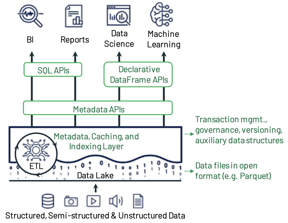
- Transactional Metadata Layer for Data Management
  - Data: stored in low-cost object storage (e.g., Amazon S3) using open file formats (e.g., Apache Parquet).
    - Challenge: Traditional data lakes lack atomic operations, making updates across multiple files complex
  - Metadata Layer (e.g. Delta Lake): Raise abstraction levels over data lake storage (e.g., S3, HDFS) to enable ACID transactions and data management features, manages transactions, versioning, auxiliary data structures, and governance over files in an open format, allowing direct data access + provide Metadata APIs
  - Benefits of Metadata Layers:
    1. Improve performance over raw data lakes.
    2. Enable data quality enforcement features: schema enforcement & data constraints (e.g., rejecting invalid records).
    3. Enhance governance: Support for access control and audit logging.
    4. Easy adoption: Can convert an existing Parquet directory into a Delta Lake table with zero copies.
- SQL Performance Optimization
  - Challenge: Traditional data warehouses achieve high performance through internal optimization (e.g., hot data storage (SSDs), indexing, and statistics), whereas Lakehouses must expose data formats for external direct data access (i.e. can not change storage formats)
  - Optimization Approach:
    - Caching: Caches frequently accessed data on SSDs or RAM for faster queries; Uses optimized transcoded formats for better performance
    - Auxiliary Data Structures: column min-max statistics in metadata for data skipping; Bloom filters and other indexing strategies to improve query efficiency.
    - Data Layout Optimizations: Ordering records for efficient access (e.g., Z-order, Hilbert curves); Optimizes column placement, compression strategies, and clustering to minimize I/O.
- Support/Efficient Access for Advanced Analytics & ML
  - ML libraries already support Parquet, so they can directly query from data lake for files in Parquet format.
  - Use Declarative DataFrame APIs (e.g. Spark SQL) for data query, which enables query to benefit from optimizations in Metadata Layer (e.g. Delta Lake).
    - DataFrame APIs map data preparation computations into Spark SQL query plans. Spark SQL lazily evaluates the transformations and passes the resulting operator plan to an optimizer, which leverages optimization features in Lakehouse
    - For Advanced Analytics wordloads: DataFrame APIs can pass input into ecosystem of advanced analytics libraries and benefit from accelerated I/O.
    - For machine learning wordloads: Spark’s query planner use SQL Pushdown Optimizations: pushes selections/projections to the Delta Lake data source, leveraging LakeHouse optimizations (e.g., caching, data skipping, and optimized data layout) for faster ML and DS workloads.
  - Challenge: Support for ML Workloads on GPUs: Some ML APIs do not push query logic to storage. Optimizing CPU-to-GPU transfers and computation overlap remains a challenge.

L11 & P11 - Geo-replication

1. Geo-replication

definition: replicate data across geographically distince locations
Benefits: fault tolerance, low latency, compliance
doubly distributed systems: replicas are distributed geographically, and (in ecah datacenter) each is itself distributed across many machines via sharding
- Sharding: put disjoint subsets of data on different servers
ALPS-Oriented Geo-Replicated Storage System - local-replica-only design: each replica is “independent”
- Reads return a current view of data from local replica; they do not examine remote replicas
- Writes are applied at local replica immediately; they return before being applied at remote replicas
- Benefit: low latency, scale out nodes/datacenter
- Drawback: weak consistency, no linearizability

2. ALPS properties

Modern web services: AP systems, at cost of linerizability (C), to provide an “always on” user experience; scalability to adapt to increasing load and storage demands => ALPS systems
A: Availability: all operations issued to the data store complete successfully. No operations can block indefinitely or return an error signifying that data is unavailable.
L: low Latency
P: Partition-tolerance: e.g. quorum-based systems ensure the “majority” partition can continue operating, thus partition tolerant, but the “minority” partition do not satisfy availability
A+P = all replicas of a system will continue to operate and be available as long as they have not failed
S: High Scalability: scales linearly (throughput and storage capacity)
sufficiently strong Consistency model
- Consistency level: strong consistency (linerizability) => causal consistency => eventual consistency
- all consistency models with a total order over operations on multiple data locations, e.g. strong consistency (linerizability, serializability, sequential consistency), are incompatible with low latency
- strongest consistency model ALPS systems can have: causal+ consistency

3. causal+ consistency (causal consistency with convergent conflict handling)

Causal consistency: data store respects the causal dependencies between operations
- Definition: potential causality: rules:
  - Thread-Of-Execution. If $a$ and $b$ are two operations in a single thread of execution, if operation $a$ happens before operation $b$ , then $a \leadsto b$ .
  - Reads-From. If $a$ is a write operation and $b$ is a read operation that returns the value written by $a$ , then $a \leadsto b$ .
  - Transitivity. if $a \leadsto b$ and $b \leadsto c$ , then $a \leadsto c$ . Thus, the causal relationship between operations is the transitive closure of the first two rules.
- Causal consistency requires that values returned from read operations at a replica are consistent with the order defined by $\leadsto$ (causality)
- Causal consistency does not order concurrent operations: if $a\not\leadsto b$ and $b\not\leadsto a$ , then $a$ and $b$ are concurrent, but if $a$ and $b$ writes to the same key, they are in conflict
convergent conflict handling: replicas never permanently diverge, and conflicting updates to the same key are dealt with identically at all sites
- use a handler function $h$ , which is associative and commutative
- example convergent conflict handling methods: Last-writer-wins, Mark as conflicting and require their resolution by some other means
- for scenarios where conflicts represent an exceptional condition that requires special handling, can only be avoided by the use of more explicit conflict resolution procedures, which require additional programmer conplexity and/or performancee overhead
System design:
1. versions are assigned to ensure that if $x_i\leadsto y_j$ than $i<j$ (notation is $\text{location}_{\text{version}}$ ). Each replica in the system always returns non-decreasing versions of a key (progressing property)
2. dependencies: $y_j$ depends on $x_i$ iff $\text{write}(x_i)\leadsto \text{write}(y_j)$ . The system writes a version only after all of its dependencies are satisfied
Causally-correct, conflict-free, and always-progressing data store
- ensures that clients see only progressively newer versions of keys
Another solution: Log-exchange-based serialization does not satisfy high scalability, as it relies on a single serilization point in each replica to establish ordering.

L12.1 - Scheduling I

Packing with uncertainty
- Overcommitting
  - monitor resource usage, identify under-utilization of allocation, and use it + assign more total “allocation” (e.g., RAM or CPU) to a machine than would fit
  - biggest issue: dealing with situations where resources run out, e.g., job tries to use its requested allocation of resources, but there isn’t enough
  - options: kill or migrate that job, kill or migrate a different job, shrink allocation
- Using slack resources: the unused capacity on a machine
  - Same issue: job tries to use its requested allocation of resources, but there isn’t enough
- (Possible) useful input to scheduler
  - Job execution plan, e.g. task DAG, inputs/outputs
  - Estimates, e.g. task durations, input sizes, transfer sizes
- VMware extra information
  - Reservation: guaranteed minimum amount (say “no” if can’t promise)
  - Limit: upper bound (so, don’t use extra resources beyond certain amount)
  - Share: relative importance of different jobs (when sharing extra resources)
- VMware constraint examples
  - Affinity: identifies VMs that would benefit from being on same machine - to allow for faster communication
  - Anti-affinity: identifies VMs that must not be on same machine - to ensure that a machine crash does not disable both

L12.2 - MapReduce Scheduling

MR Network Topology
- Data Center: Core switches - End of Row switches - Top of Rack switches
- bandwidth between two nodes is dependent on their relative locations: closer, larger
MR Scheduling Architecture
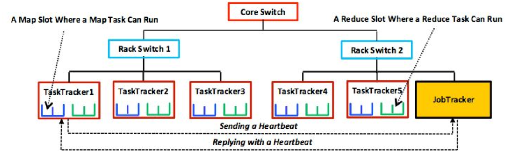
- One master, JobTracker: combines updates to produce a global view
- One or many slaves, TaskTrackers: have configurable number of Map or Reduce task slots (default, 2M, 2R)
  - TaskTrackers send a heartbeat (containing progress, if allocated task(s)) to JobTracker every 5 secs
MR Job Submission
- runJob creates JobClient and submits Job to JobTracker
- JobTracker adds to queue
- When TaskTracker sends heartbeat to JobTracker indicating its free, Scheduler chooses a task from job
MR Scheduling
- Task scheduler (schedule tasks within job)
  - policies
    - Fills Map slots before Reduce slots; If no empty map slot, choose next reduce task
    - Map: locality - Pick a Map task whose split is close to TaskTracker’s network location, closest is data-local
    - Reduce: next task
  - Considerations: Data-locality; Variations in overall system workloads; Failure
  - Pull scheduling strategy: TaskTracker pulls tasks by making requests
- Centralized job scheduler (scheduling multiple jobs)
  - Default: FIFO - An MR job consumes all cluster resources
  - Fair Scheduler - Each user gets a pool. All pools get an equal share of cluster resources. Jobs within the pool share resources equally
  - Capacity Scheduler - Creates job queues. Each queue is configured with capacity (a number of slots or a percentage of cluster resources). Within a queue, scheduling is priority-based
Hadoop Fault Tolerance
- faulty nodes, corrupted files - storage layer replicas (default is 3)
- Task Resiliency (task slowdown or failure)
  - Speculative Execution
    - monitoring, replication
    - Locating Straggler: a task’s progress score is less than (average – 0.2), and the task has run for at least 1 minute
    - speculative tasks: lowest prioritization
    - drawbacks
      - lots of speculative tasks in heterogeneous environments or due to transient congestion
      - Blind Speculative Task Launch: Launches speculative tasks at TTs without checking the speed of TT or the load of speculative task, making slow TT will become slower
      - Hadoop often prefers data locality over speed.
      - The three reduce stages are treated equally, but the shuffle stage is typically slower than the merge & sort and reduce stages
  - TT failure: JT asks another TT to re-execute all Mappers that previously ran + were in progress on the failed TT
  - Task failure: reschedule a task on another TT (blacklist current TT). If the task fails >4 times, job failure

L13 - Kubernetes

Cloud-Native Applications
- auto-scaling, design for failure, modularity, API-driven composition, automation
- Kubernetes: Cloud-Native Orchestration Frameworks
k8s Architecture
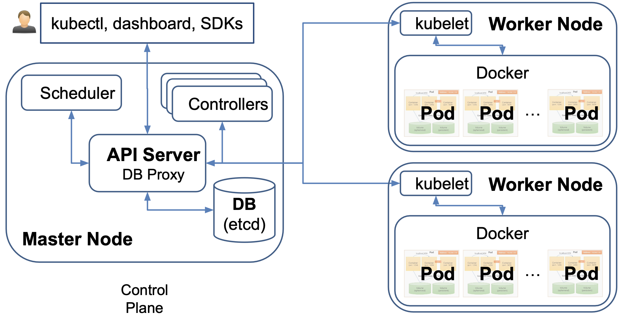
- Pod: One or More Containers + Resources + Labels
  - Multi-Container Pods: Scaling/replication unit: runtime components that must run together
    - Sidecar pattern: “secondary” functions deployed in separate containers
    - Ambassador/Proxy pattern: simplify access to an external system
    - Adapter pattern: simplify access from an external system
- Deployments & Desired State
  - User sends a Deployment object (written in YAML) to the API Server
  - A Deployment provides declarative updates for Pods & ReplicaSets
  - A desired state is described in a Deployment
  - The Deployment Controller changes the actual state to the desired state at a controlled rate
k8s Composite Application Types: Deployment (Replica set), Daemon Set, Stateful Set, Job, Custom, …
k8s default scheduler
- Main goal: placement of Pods on Nodes - Triggered primarily by watching for new Pods in ‘pending’ state
- FIFO scheduling
- Supports priority-based arbitration and eviction
- Placement Policies
  - Filter() (predicates) - e.g. PodFitsResources, PodMatchNodeSelector (labels match), MatchInterPodAffinity (Affinity: same host/rack/zone/etc, Anti-Affinity)
  - Prioritize() (utility functions) - e.g. InterPodAffinity, Least/Most/BalancedResourceAllocation, ImageLocality

L20G - Cost Optimization and Workload Disruption in Kubernetes

Workload Disruption = a condition in which a workload experiences degradation in (one or more):
- Performance (e.g., longer response times due to CPU throttling),
- Availability (e.g., temporary outage due to zero available replicas in a workload), or
- Reliability (e.g., errors due to sudden termination of a Pod)
- Reasons: spot interruptions, imperfect scale-up/down
Kubernetes handles Spot interruptions
- ‘cordon’ the node: no new pods can be scheduled on it
- graceful eviction: node draining
  - honoring Pod Disruption Budgets (PDBs), etc.
  - terminate eligiable pods
  - wait for Termination Grace Period for all Pods (default 30s), if after that containers are still running, force kill
- force-terminate remaining pods
- Recommendations
  - make your applications ‘spot-friendly’
    - Tolerant to evictions: graceful shutdown, termination grace period, PDB
    - Short termination grace period (< 2 min)
    - Short Startup time
    - Configure microservices which are not ‘spot-friendly’ to run on non-spot instances
Pod Disruption Budgets PDB: defines how many replicas of an application can be temporarily unavailable during a voluntary disruption (maxUnavailable)
- Ensure safe node draining (e.g., during upgrades or spot interruptions) without application downtime.
- Prevent too many pods of the same application from being evicted at the same time. Ensure that a minimum number of healthy replicas continue to serve users.
- Configuration: PDB (e.g. maxUnavailable, etc.), Pod Termination Grace Period, Container “readiness” probe
- Workflow: pod eviction -> find PDB by Label Selecter -> trigger pod termination only if setisfies PDB predicates (e.g. currentHealthy > desiredHealthy)
Resource Allocation in Kubernetes
- pod (container) have specification of Requests and Limits for CPU and Memory
- Scheduler: ensures that the sum of requests (across all the containers) of a Pod match the free capacity of the node
- challenges
  - Developers often don’t know how much resources each container will actually need
  - Applications often do not behave well under resource pressure
  - the availability of resources beyond “requests” is non-deterministic
  - common (mis)perception that “requests” should be set according to “typical” demand, and “limits” should be set according to peak demand during spikes
- Recommendations to minimize workload desruption
  - Start with an assumption that requests=limits
  - Invest in understanding the resource demand patterns for your application
  - Monitor resource utilization and workload disruption (e.g., due to OOM)
  - Consider using automated tools
Horizontal Pod Autoscaling - Recommendations
- scale-up not fast enough to accomodate the spike => set target low enough to allow ‘headroom’ during spikes, aligned with the replica startup time
- Uneven load balancing hide load spikes => ensure even load balancing across replicas
- Redisness timeout too small, so now Pod get killed before finishing initialization => implement readiness probes, make sure application start quickly
- Non-graceful application shutdown, causing workload disruption on scale-down => implement graceful shutdown
Vertical Pod Autoscaling - Recommendations
- To little/much ‘headroom’ leading to throttling/ waste => leverage automated tools to adjust resource allocation dynamically
- Different applications might have different levels of sensitivity to throttling, for each of the resources => find a tradeoff between cost and throttling which is optimal for your application
- Behavior (and resource demand) of each replica might change regardless of changes in external load (e.g. due to startup, periodic jobs, etc.) => analyze resource usage trends over time to find seasonality, correlations between workloads; decouple the application into runtime components with consistent resource usage (per load unit)
- “noisy neighbors” => co-locate workloads with negative correlation in load over time
Cluster Autoscaling
- Scale-Up: Dynamically provision new node(s) that match the requirements of pending pods (CPU, Memory, node labels, etc)
- Scale-Down: Detect low utilization of nodes (e.g., following a decrease in load, and removal of replicas of some workloads), Trigger ‘consolidation’ to fewer or smaller/cheaper nodes
- Recommendations:
  - spot interruptions => define Topology Spread for the workload, to minimize disruption due to interruption of one or more nodes

L14 - Scheduling II: Multi-level Scheduling

Cluster Scheduling with multiple frameworks (programming models): heterogeneous mix of activity types; heterogeneous machines
- one monolithic scheduler:
  - Advantage: can (theoretically) achieve optimal schedule
  - Disadvantages
    - Complexity - hard to scale and ensure resilience of scheduler
    - Hard to anticipate future frameworks’ requirements - Scheduler can only consider what it is programmed to consider
    - Need to refactor existing frameworks to yield control to central scheduler
- Two-level scheduling
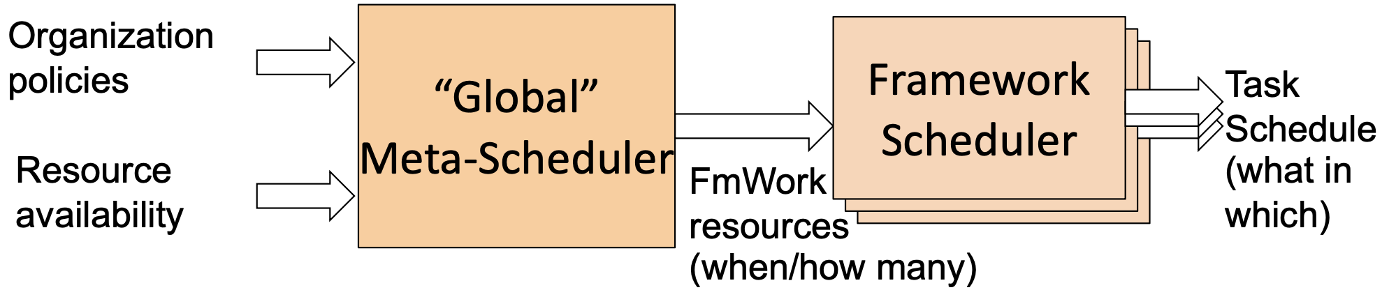
  - Advantages:
    - Simple - easier to scale and make resilient
    - Easier to port existing frameworks, support new ones
  - Disadvantages:
    - Distributed scheduling decision - may be suboptimal
    - Need to balance awareness with coordination overhead
Two-level schedular: Mesos - resource offers
- Vector of available resources on a node, E.g., node1: <1CPU, 1GB>, node2: <4CPU, 16GB>
- Meta-scheduler sends resource offers to frameworks
- Frameworks select which (if any) offers to accept
- Task scheduling in frameworks
- allocations are done one-at-a-time without consideration of other pending jobs and there is no mechanism to resolve conflicts between jobs of equal priority; can also revoke (kill) tasks
- challenges
  - Allocation changes - How should the meta-scheduler arbitrate among framework schedulers?
  - Planning ahead - lack of central planning of schedule can lead to distributed hoarding
  - Limited visibility for frameworks into overall cluster state
Distributed schedular: Omega - shared state
- Expose (and update) cluster state and schedule to all framework schedulers
- Let each framework make and enact decisions independently
- Supports Scheduling into the Future (Backfilling)
  - A scheduler can reserve future slots for a hard-to-schedule job without blocking the entire schedule.
  - Meanwhile, other jobs can be backfilled into earlier, unreserved slots.
  - This avoids the “greedy grab and wait” behavior that causes distributed hoarding
- challenges
  - performance overheads in maintaining shared state
  - can repeat work
  - Allocation changes - how to arbitrate?

L15 - YARN Scheduling

YARN Architecture
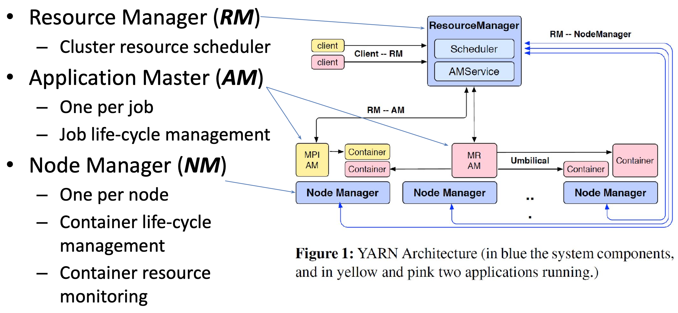
- One Master Node with RM
  - Tracks resource usage and node liveness
  - Scheduler
    - request-based scueduler, support fair / capacity scheduling (locality)
    - Dynamically allocates leases to applications
  - Application manager: manages running the AM
  - When a job is submitted, the RM assigns a jobID to it and allocates a container to run the corresponding AM
  - Interacts with NM to assemble a global view
  - Can reclaim allocated resources by
    - Collaborating with AMs
    - Killing containers directly through the NM
- Multiple Slave Nodes, each with NM
  - Container represents a lease for an allocated resource in the cluster
    - includes details such as: CountainerId (globally unique), NodeId, Resource allocated, Priority, ContainerState, ContanerToken, ContainerStatus
  - manages container lifecycle
    - Authenticates container leases
    - Allocates container to applications
    - Reports usage through heartbeat to RM
    - Kills containers as directed by RM or AM
  - monitors containers
- AM: one per job
  - Manages the lifecycle of a job: starting, monitoring, and restarting tasks
  - Creates a logical plan & physical plan of the job
  - Requests resources through a heartbeat to the RM; Receives a resource lease from the RM
  - Coordinates execution: Each task runs within a container on each NM
  - Plans around faults
YARN interfaces
- Client-RM Protocol: This is the protocol for the client to communicate with the RM to launch a new job, check on the status of the job, and/or kill a job
- AM-RM Protocol: This is the protocol used by the AM to register/unregister itself with the RM, as well as to request resources from the RM scheduler to run its tasks
  - Resource Request: <priority, (host, rack, *), resources, #containers>
- AM-NM Protocol: This is the protocol used by the AM to communicate with the NM to start/stop containers
- NM-RM Protocol: This is the protocol used by the NM to communicate its status to the RM
- RM is blind to the tasks running within an application
- AM has no view of other running applications
YARN Scheduling
- FIFO Scheduler
- Fair Scheduler: Has multiple queues and tries to fairly allocate resources to the queues, Dominant Resource Fairness algorithm
- Capacity Scheduler: Has multiple queues and tries to allocate resources to the queues such that each queue’s capacity constraint is not violated
- Scheduling: Resource manager has an asynchronous schedule thread, which gets a random node from the list of nodes maintained by the resource manager and tries to schedule an application’s request on to the node
- does not support multi-application environments where custom, app-specific scheduling policies are critical, e.g. gang scheduling
YARN Fault Tolerance
- RM Failure: Single point of failure, Can recover from persistent storage (kill all containers including Ams)
- NM Failure: detected by RM through heartbeat timeout and report to AMs. AMs responsibility
- AM Failure: RM restarts AM, AM has to resync with all running tasks or all running tasks are killed
- Task failure: Framework (AM) responsibility

L16G - Moirai: Optimizing Placement of Data and Compute in Hybrid Clouds

Motivation:
- Jobs
  - Outputs of analytics jobs are much smaller than their inputs - transferring outputs back to users is lightweight
  - On-prem is paid for, cloud follows a pay-as-you-go model - make full use of on-prem compute resources
- Data
  - Fixed cost based on bandwidth and lease duration - Usage must stay within the allocated bandwidth
  - Data movement: ingress is free, egress in expensive
- In Hybrid cloud, egress cost is the dominant factor - want to minimize egress cost
- Unoptimized Placement -> High Costs
  - remote access - usage on network links
  - replicate dataset in advance - extra cloud storage cost
Moirai: minimizes cost by solving a mixed integer programming problem, using heuristics
- Heuristic 1: Group Similar Jobs
  - Where are datasets of a job located
  - how much data a job access from each dataset
  - group recurring jobs into one logical job
- Heuristic 2: Remove Inactive Datasets
- Heuristic 3: Make Dependency Graph Sparser
  - by replication: Preselect datasets to replicate before optimization

L19G - Sia: Using GPUs during pipeline bubbles with heterogeneity-aware cluster scheduling

Goal: minimize job completion times (JCT) for DL Training jobs
- Assumption: JCT for DLT jobs not known ahead of time
- Users choose batch size + resources (i.e., # and type of GPUs) at job submission time
- optimize allocation + placement
Strategy: configs restrict the space of allocations
- Configuration := (# nodes, # GPUs, GPU type+topology)
- Many-one map: many topology-aware placements = one config
Large Model Training
- Data Parallelism
- Pipeline Parallelism
- DP + PP: DP/scale-out increases pipeline bubbles (bubble ratio)
- Solution: run other jobs during bubbles: bubble instruction
- challenges:
  - GPU memory management
  - context-switching
  - Scheduling

L21G - Microsoft Singularity/Project Forge

L17 - Diagnosis via Monitoring and Tracing

data gathering methods on the cloud
1. Monitoring via performance counters
  - aggregates of low-level data, e.g. CPU time, disk IOs
  - Pros: Lightweight, commonly available
  - Cons: Black-box; aggregates; per-“node”
2. Logging events of interest
  - detailed text describing system’s behavior
  - Pros: White-box approach
  - Cons: High overhead; per-“node”
3. End-to-end activity tracing
  - worklofw-based logging
  - Pros: White box, distinguishes workflows
  - Cons: Requires software modifications
Ganglia: Monitoring [type 1]
- Designed for HPC environments, assumes bare-metal hardware
- Collects and aggregates counters
  - Counters can be app or machine specific
  - Within cluster, counters visible everywhere
  - Counters from multiple clusters aggregated
- Architecture
  - gmond (Ganglia Monitoring Daemon) - Runs on every node; collects and sends local metrics
  - gmetad (Ganglia Meta Daemon) - Poll and Aggregates metrics from multiple clusters; stores data
  - Web Frontend - Visualizes metrics
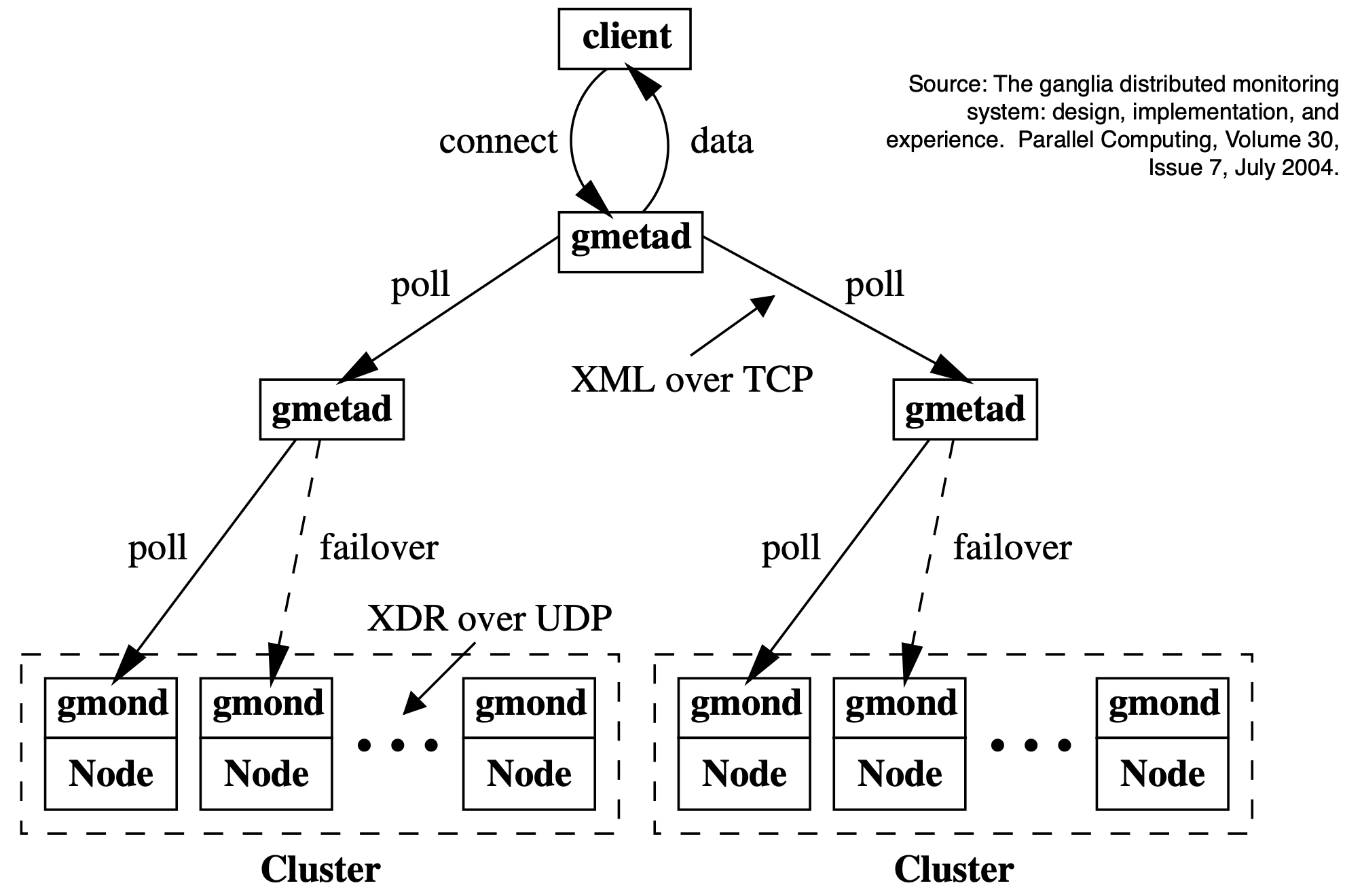
End-to-end tracing [type 3]
- reveals causality-related activity, i.e., the sequence and interdependencies of actions across services
- Trace: Defined as a set of events (spans) across threads or machines, merged and ordered by causality
- Use case: Enables analyzing how individual requests flow through a distributed system
- Implementation: Trace points are hooked into services/components that a request touches
  - Start traces: a new user request arrives => assign a trace ID
  - Propagation: Trace ID is passed downstream to all involved services/components
  - Trace reconstruction: Logs from multiple services are stitched together using trace IDs to reconstruct full workflows
- Challenge:
  - Tracing is less accurate with asynchronous or batched work.
  - Causality becomes harder to track when request paths are non-linear or parallel.
- trace every request is too expensive => Use sampling to reduce overhead
  - byte limit per trace span
  - request-level sampling
Dapper: End-to-end tracing [type 3]
- Traces are trees of Remote Procedure Calls (RPCs): node is activity, edge is causal link
- Sample at request entry (based on hash of root ID)
Spectroscope: End-to-end tracing analysis tool
- Identify root causes of performance degradations by ID’ing changed request flows
- Output:
  - Groups of before/after request flows
  - Automatic identification of structural or latency-based changes
- Workflow: grouping, change identification (structural + response-time change), ranking, presentation
  - Response-time changes: Flow is structurally identical. Detected using statistical significance testing (e.g., t-tests on latency)
  - Structural changes: Detected using heuristics like frequency of specific trace types

L18G - Amazon Redshift

Security and Availability: Multi-AZ highly resilient data warehouse, auto-failover w/o data loss
Performance: query optimizations, co-located join, reduction of shuffling, cache compilation (Compilation-as-a-Service), string compression encoding
Storage and Compute Elasticity: separate compute and storage (scale independently)
- Compute Elasticity Improvements:
  - traditional method: stopping the cluster, redistributing all data across nodes, and then restarting
  - Redshift: only moves partitions in a whole to avoid data redistribution, preserves existing data slices and only redistributes metadata or small portions
- Data sharing with auto-scaling, across the globe
  - optimized through local caching and optimized query routing
Autonomics and Serverless
- auto maintenance (table optimization, analyze, vacuum, materialized view refresh)
- auto workload management (short query acceleration, query predictor)
- serverless
- AI-driven
Integrations
- traditional method: manual data pipelines
- Redshift: zero-ETL: streaming ingestion (real-time analytics), automated file ingestion from Amazon S3, integration with Amazon Aurora MySQL etc.
Comprehensive Analytics and ML: fast migration, SUPER data type for semi-structured data, train and create ML models using SQL

L22G - Cloud Co-location and Attacks on Public Cloud

Infrastructure Security of cloud infrastructure: physical access, media sanitization, data protection (encryption)
- Hardware: e.g. Google Titan Chip
Sandboxing: confinement - split attack surface into smaller domains
- Hardware: expensive
- OS - container - VM
  - reference monitor
- process
- Threads: e.g. Software Fault Isolation (SFI) Isolating threads sharing same address space
- Application level confinement: e.g. Browser sandbox for Javascript and WebAssembly
Attack on cloud Step 1: collocation - attacker collocates malicious VM/containers on the same physical machine they want to attack
- Prevent: Sandboxing: do not leak host info to the collocated attacker
- but, Attacker use side channels to figure out collocation
  - attacker can bypass software countermeasures by directly interacting with the shared underlying hardware (e.g., to get the host fingerprint)
  - Side-channels everywhere (CPU, Memory, e.g. host’s boot time)
  - Host fingerprints are highly accurate and long-lasting
- Instance Placement Policy: High container usage can trick Cloud Run to spread instances across many hosts, Allow attackers to go beyond their base hosts
- Prevent: Hardware virtualization offers an opportunity to block side-channel leakage, but we need to carefully configure the hypervisor
Spectre: break confinement
- e.g., trick the CPU to run the mispredicted branch
encrypted AI
- Data must be encrypted at rest and in transit, but computation on plaintext in cloud environments remains a vulnerability
- encrypted AI, but Massive compute and memory overhead + scalability challenge